Dissecting ThunderKittens: Anatomy of a Compact DSL for High-Performance AI Kernels

21 May, 2026

Introduction

Modern ML workloads depend heavily on custom GPU kernels. Even when a model is expressed as clean tensor operations, the performance almost always comes from specialised implementations underneath. Good examples of this are the many different attention mechanisms, GEMMs across different precisions, and MoE-style grouped GEMMs, which have become a fairly common architectural choice in state-of-the-art models nowadays.

This matters a lot if we look at it from the perspective of scaling laws. Better models have generally come from some mix of better algorithms, more data, and more compute. If we want to keep pushing that forward, we care not just about algorithmic quality, but also about how efficiently those algorithms actually run on hardware. One clean way to frame it, as Tri Dao puts it, is:

We want to improve both terms. On the algorithm side, researchers need to iterate quickly on new architectures and new training and inference recipes. But for any of that to matter at scale, it has to translate into code that actually runs fast on real hardware. There is a persistent tension here: we want programming environments productive enough for research, but close enough to the metal to get serious performance and scale well.

This is the space GPU programming DSLs occupy, and they span a pretty wide range.

At the high end, frameworks like PyTorch let researchers write tensor expressions without thinking about the GPU at all. The framework handles kernel dispatch, and with PyTorch 2, TorchDynamo + TorchInductor can generate competitive GPU code, often by emitting Triton. One level lower, Triton gives more explicit control over tiling, memory access patterns, and program structure, while still hiding most CUDA complexity. Go lower still, into CUDA C++, CUTLASS/CuTe, or PTX, and we get direct hardware control, but now we are managing memory layouts, warp synchronisation, tensor core scheduling, and a lot of boilerplate.

The deeper we go, the more of the GPU hierarchy we can reason about, but the more expertise and code it takes to do anything.

ThunderKittens, an embedded DSL inside CUDA from Stanford's Hazy Research Lab, sits at a genuinely interesting point on this spectrum. The research question behind it is clean: how small can a programming abstraction be while still supporting fast kernels across a broad range of AI workloads? Rather than hiding the hardware or exposing all of it, TK finds a middle ground: it abstracts the repetitive plumbing — tile layouts, shared memory allocation, register fragments, TMA tensor maps, tensor core descriptors — while still leaving us close enough to reason carefully about what data moves where, how the pipeline stages, and how the work gets scheduled. And since it is embedded in CUDA, we can always drop down to raw CUDA or inline PTX when we need something the library does not expose.

That is the framing I want to use in this post. I want to understand what abstractions TK exposes, why they look the way they do, and how they map onto Hopper and Blackwell GPU hardware.

We will start from the core programming model: global layouts, shared tiles, register tiles, vectors, compute wrappers, and memory movement. Then we will look at the newest Blackwell-specific additions: tcgen05, 2xSM MMA, tensor memory, and Cluster Launch Control. Finally, we will make it all concrete by building an attention prefill kernel using TK's lcf pipeline template and benchmarking it against FlashAttention-2 and 3.

ThunderKittens Programming Model & Core Abstractions

Before going deeper, it helps to first step back and ask what ThunderKittens is actually trying to do.

At a high level, TK provides an opinionated set of abstractions that map well to AI kernels. Instead of writing everything directly in raw CUDA, TK lets us work with tiles and higher-level operations over those tiles. Many of these operations feel somewhat similar to PyTorch primitives, which gives a familiar feel to kernel development for people coming from an ML background.

That is really the central idea behind the framework: reduce the complexity of writing high-performance kernels without giving up the control needed to reach modern GPUs efficiently.

As the paper puts it:

“Despite the apparent need for a myriad of techniques to leverage all these hardware capabilities, our central technical finding is that indeed, for many AI kernels, a small number of key abstractions exist that can simplify the process of writing high-performance kernels.”

Before we can really appreciate that claim, it is important to have a solid mental model of the GPU hardware itself. If concepts like warps, thread blocks, shared memory, tensor cores, and occupancy do not already feel intuitive, I would strongly recommend first reading the opening sections of my H100 GEMM optimisation post. For the newer Blackwell components, we will discuss them in this blog, so bear with me on that. With that foundation in place, the TK programming model becomes much easier to reason about.

From there, we can start looking at the core abstractions that ThunderKittens builds around, and why they map so naturally onto modern GPU hardware. As a quick refresher, here is the GPU memory hierarchy and its corresponding CUDA programming model alongside TK's tile abstractions (excuse my awkward triangle):

We can now see how TK’s tile abstractions fit into this view of the memory hierarchy. Tile abstractions are the fundamental building blocks of the TK programming model; all of the other components are layered on top of them. At a high level, the main ThunderKittens abstractions look like this:

Tile Abstractions

TK is built around the idea that everything should be expressed in terms of tiles that map cleanly onto the GPU hierarchy. At its most basic, TK uses a base tile with a fixed height of 16, while the width depends on datatype. For fp16, bf16, and the other 16 column cases, that base tile is 16×16. For 1 byte types such as fp8, it becomes 16×32. This was not an arbitrary choice. It follows directly from how tensor core instructions expose their fragments, and from how those fragments need to be staged through shared memory.

We can already see this in older tensor core instructions. In SASS, HMMA instructions often operate on shapes such as 16×8×16 or 16×8×8, so even if the hardware instruction itself is not literally a square 16×16 multiply, the 16 extent is still very real in the fragment layout. On Hopper, the warp group version shows up as HGMMA, with much larger shapes such as 64×256×16. So the point is not that every tensor core instruction is exactly 16×16. The point is that the hardware exposes a very strong 16 based structure, and larger fragments are built by composing repeated pieces of that structure.

The datatype dependence becomes especially clear once we look at Hopper WGMMA input fragments. For 16 bit inputs, the m64nNk16 family naturally exposes a 64×16 input slab, which TK can treat as repeated 16×16 pieces. For fp8, the corresponding family is m64nNk32, and now that same input side widens to 64×32. This is exactly why TK keeps the row granularity fixed at 16, but allows the column granularity to widen for 1 byte types. The abstraction is still the same one, but the hardware fragment it is built around is now wider.

So when TK builds larger tiles, the easiest way to think about it is as stacking these base fragments until the full tile shape is covered. A larger 16 bit tile such as st_bf<64,64> can be viewed as a 4×4 arrangement of 16×16 fragments. An fp8 tile such as st_fp8e4m3<64,64> instead becomes a 4×2 arrangement of 16×32 fragments. This is a useful way to reason about the shapes TK works with, even though a shared tile itself is still stored as one shared memory object.

One small caveat before we move on: TK does not try to expose every numerical format that Hopper or Blackwell supports in hardware. In the current repo state I am looking at (commit #01cb68c), the main tile types cover the formats TK actually builds around: bf16, half (FP16), float (FP32), the usual FP8 formats fp8e4m3 and fp8e5m2, Blackwell’s fp8e8m0, and packed FP4 storage such as fp4e2m1_2.

FP4 is the one that needs a little extra care in our mental model. TK does define a scalar fp4e2m1 type, but tile types use packed storage, because a single FP4 value is only 4 bits. Two FP4 values fit naturally into one byte, so the tile-facing type is something like fp4e2m1_2. That means packed FP4 still looks like a 16×32 base tile in TK’s addressable tile units, but if we count the actual individual FP4 values, that same tile represents 16×64 scalars. So the general rule still holds, we just have to remember what “one element” means once the datatype itself is packed.

This is the key idea. TK’s tile shapes fit naturally with tensor core style matrix fragments, not because every instruction is literally a single square tile, but because they provide a clean software unit for composing the larger fragments the hardware actually works with. That is already visible in older HMMA style instructions, where the 16 granularity is obvious, and it remains true on Hopper HGMMA instructions, even though the full warp group operation is much larger. So when TK builds something larger, it is not forcing an awkward abstraction onto the GPU. It is simply composing larger tiles out of smaller pieces that already match how the hardware wants to work.

In practice, TK builds its programming model around three core tile-level abstractions: global layout descriptors (gl), shared tiles (st), and register tiles (rt). Alongside these, it also provides shared and register vector abstractions (sv, rv) for kernels that are more naturally expressed in vector form, think for example of LayerNorm or RMSNorm.

That said, TK 2.0 is now mainly built and tested for Hopper and Blackwell GPUs. The project specifically states that it no longer actively supports Ampere.

Before looking at the individual abstractions in more detail, it is useful to quickly note a few general constants and thread indexing helpers that appear throughout the TK codebase. These are usually accessed directly as kittens::xxx.

This is a much cleaner foundation for the rest of the section, because now the later abstractions can be read in terms of that same underlying idea: TK keeps the row granularity fixed at 16, lets the width follow the datatype, and then builds larger shared and register level objects by composing shapes that already match the hardware’s fragment structure.

1. Register tiles: Register tiles are the main abstraction TK uses for values that live in registers during compute. In GEMM style kernels, these are very often the tiles that hold the accumulator fragments, which is why register tiles show up so prominently around tensor core instructions. In the source, the general form is rt<T, rows, cols, layout>, so the type is parameterised by datatype, shape, and layout. In practice, though, we will usually see the shorter aliases such as rt_fl<M, N> for an FP32 register tile or rt_bf<M, N> for a BF16 register tile.

Under the hood, register tiles follow the same "building blocks" story we introduced above. The row granularity stays fixed at 16, while the width depends on datatype. In rt_base.cuh, the base register fragment uses TILE_ROW_DIM<T> and TILE_COL_DIM<T> directly, and then in rt.cuh larger register tiles are formed explicitly by composing those base fragments into a 2D grid:

rt_base<T, layout> tiles[height][width]

So, for example, an rt_fl<64, 64> is internally a 4×4 grid of 16×16 base register fragments. For fp8 register tiles, the same idea still holds, except the base fragment widens to 16×32, so the resulting grid changes accordingly. This is one place where the register tile abstraction is especially clean: unlike shared tiles, which only admit this interpretation logically, register tiles are literally represented in the source as a grid of datatype-specific base fragments.

This datatype dependence becomes especially important when TK has to convert between register tile types. It is tempting to think of this as just casting each value independently. But for tensor-core register fragments this is more complex. The values are not sitting in one thread as a simple contiguous array. They are already distributed across lanes in the layout expected by the hardware like we saw in the earlier visuals.

For 16-bit types such as fp16 and bf16, a 32-bit register naturally packs two values. For fp8, the same 32-bit quantity packs four values. So an fp8 register fragment is not merely a smaller version of the bf16 fragment. It has a different per-lane ownership structure.

This is why converting a register tile from bf16 or fp32 into fp8 is really three operations at once: convert the numerical format, repack pairs into four-value fp8 groups, and move values between lanes so that each lane ends up with the fragment shape the fp8 tensor-core path expects. Let's have a go at this visually to make it more concrete.

In the 16-bit style layout, lane T2 may own a pair of values and lane T3 may own the next pair. But in the fp8 layout, one destination lane needs a four-value pack. So the fp8 lane cannot be filled by only casting its own local pair. It has to gather values that originally lived in neighboring lanes, repack them, and only then store the result as a packed fp8 fragment. This is why TK’s fp8 conversion path uses shuffle instructions instead of just applying a scalar cast independently inside each lane. Feel free to check out the code as well for the conversion function.

There is one more important detail here. A register tile in TK is a logical tile, not a private per-thread matrix. Physically, its entries are distributed across the registers of the lanes participating in the warp. Each thread holds only its own fragment of that larger logical object. This matters a lot for understanding both MMA style instructions and the vector abstractions we will get to later, because many of the operations in TK are really acting on register fragments spread cooperatively across the warp rather than on one thread-local array.

On Hopper, this becomes especially concrete for warpgroup GEMMs. The full accumulator fragment for a WGMMA instruction may cover a 64×N tile, but that accumulator is still distributed across the 128 threads of the warpgroup. Each warp owns a 16 row slice, and together the four warps realise the full output tile. So when we look at a register tile in this setting, we should think of it not just as “a tile in registers,” but as a warp-distributed tile in registers.

2. Shared tiles: If register tiles are the compute side abstraction of TK, shared tiles are the staging abstraction. Their role is to hold data in SMEM after it has been fetched from GMEM, but before it is consumed by the compute path. Sometimes that means a warp loads the data from SMEM into register fragments using instructions like ldmatrix. On Hopper WGMMA, it can also mean the tensor core instruction consumes the SMEM tile through a matrix descriptor, while accumulating into register tiles. Either way, shared tiles are where TK organises data so the GPU can reuse it efficiently and feed the compute instructions in the layout they expect.

The core type is defined as st<T, rows, cols, swizzle, swizzle_bytes>. The most important thing to notice is that a shared tile actually owns storage, hence the source:

dtype data[rows * cols]; ///< Raw data storage for the tile.

So shared tiles are not descriptors or views. They are real SMEM objects that own tile-shaped storage. The “building blocks” narrative we have been using still applies here, but more as a logical way to reason about the shape of the tile. Physically, the shared tile itself is stored as one shared-memory object.

The st type also defines an idx(...) helper, whose job is simply to answer the question: if I want the element at row r and column c of this shared tile, where exactly does that live in shared memory? In the simplest case, where the tile is laid out as an ordinary row-major array, that address is just the familiar r * cols + c.

TK also supports swizzled SMEM layouts. Swizzling changes the physical addresses in shared memory while preserving the same logical tile coordinates. We still ask for (r, c), but the address returned by idx(...) may no longer be the naive row-major location. This matters because shared memory is banked, and the wrong access pattern can cause many threads to contend for the same banks at the same time. TK supports specialised 32, 64, and 128-byte swizzle patterns to reduce, or sometimes eliminate, those bank conflicts Shared memory on NVIDIA GPUs, including H100, is divided into 32 banks, and each bank can serve one 4-byte word per cycle. I like to think of it as thirty two checkout lanes at a supermarket: if every thread goes to a different lane, everyone gets served together.

A bank conflict happens when multiple threads in a warp access different addresses in the same bank. In that case, the hardware cannot serve all of those requests at once, so it has to serialise them across multiple cycles. In Nsight Compute terminology, the SMEM request gets split into multiple wavefronts. A conflict free access needs fewer wavefronts; a conflicted access needs extra wavefronts, which is where the stall comes from.

There is one important exception: if multiple threads read the exact same address, the hardware can broadcast that value instead of treating it as a normal bank conflict. So the bad case is not “many threads touch the same bank” by itself. The bad case is “many threads touch different addresses inside the same bank.” .

__device__ static inline T* idx(T *ptr, int2 coord) { // naive row-major coord default
    int r = coord.x, c = coord.y; // alias
    if constexpr (swizzle) {
        static constexpr int swizzle_repeat = swizzle_bytes * 8;
        static constexpr int subtile_cols = swizzle_bytes / sizeof(T);
        const int outer_idx = c / subtile_cols;
        const uint64_t addr = (uint64_t)(&ptr[outer_idx * rows * subtile_cols + r * subtile_cols + c % subtile_cols]);
        const int swizzle = ((addr % swizzle_repeat) >> 7) << 4;
        return (T*)(addr ^ swizzle);
    } else {
        return &ptr[r * cols + c];
    }
}

The key idea is that we continue to think in terms of logical tile coordinates, (r, c), while idx(...) maps those logical coordinates to the correct physical address in SMEM depending on the layout we choose. If the tile is not swizzled, this collapses to ordinary row-major indexing. If the tile is swizzled, the helper applies the address transformation for us.

This helper is mostly relevant for ordinary reads, writes, and smaller manipulations of a shared tile. Bulk hardware paths such as TMA and WGMMA do not simply call idx(...) for every element; they rely on tensor maps or matrix descriptors built from the tile metadata. But the conceptual role is the same: TK lets us keep thinking in logical tile coordinates while the library handles the physical shared-memory layout needed by the hardware.

For WGMMA, one important rule is that matrix A can live either in registers or in shared memory, but matrix B must live in shared memory. So the layout of SMEM operands matters a lot.

Conceptually, we can think of each SMEM matrix as being broken into smaller core matrices. During WGMMA, the SMEM operands are consumed through these core-matrix-sized pieces, rather than as one giant matrix all at once. For 16-bit types such as bf16 or fp16, the core matrix is 8×8. For fp8, it becomes 8×16, because each element is half the size.

Let’s visualise a 16-bit 64×64 matrix A tile residing in SMEM.

Small note on the bottom layout figures: these are not drawn at the scalar bf16-element level anymore. Each cell is a 16B chunk, which for bf16 means 8 scalar values. So one column in the bottom figure corresponds to one 8×8 bf16 core matrix: 8 rows, with each row compressed into one 16B chunk. The full bottom figure therefore shows one 8×64 band of the larger 64×64 tile, not the whole tile. If we wanted to draw the full tile in this chunk view, it would be 64×8 chunks. I only draw one 8-row band to keep the swizzle pattern readable and easier for me to draw.

Each 16B chunk spans four SMEM banks, because each bank serves one 4B word per cycle. In the naive layout, the first 16B row chunk from each of the eight rows lands on the same four banks. So logical chunk column 0 maps to banks 0, 1, 2, and 3 for every row. Since those are different addresses hitting the same bank group, the hardware has to serialise them, giving an 8-way bank conflict in this simplified view.

With 32B swizzling, the same logical chunks are spread across two bank groups instead of one. The first four row chunks still hit one bank group, but the next four hit another, reducing the conflict from 8-way to 4-way. With 64B swizzling, they are spread further, reducing the conflict to 2-way. With 128B swizzling, this simplified view shows the chunks spread across all the bank groups, removing the conflict for this access pattern.

The byte width also explains the datatype-dependent tile width. To form one full 32-byte swizzle region across a row, a 16-bit tile needs at least 16 elements across the column dimension: 16 elements * 2B = 32B.

For fp8, each element is only 1 byte, so the same 32B swizzle region requires 32 elements: 32 elements * 1B = 32B

So fp8 needs at least 32 columns to form the same 32B swizzle region. This ties back to why TK’s fp8 base tile width is 16×32, while the 16-bit base tile is 16×16.

The same logic applies to the larger swizzle modes. A 64B swizzle region corresponds to 32 bf16/fp16 elements, while a 128B swizzle region corresponds to 64 bf16/fp16 elements. For fp8, those same regions correspond to 64 and 128 fp8 elements. That does not mean the base tile itself has to be that wide, but to use those larger swizzle modes, the shared tile must be wide enough, or be a multiple of the required width, so the hardware has a full byte-region to swizzle over.

We can see the swizzling choice TK makes for us being aware of the tile shape we require. If we don't manually specify a swizzle size, TK chooses one from the tile width and datatype:

// If a user specifies a swizzle bytes value, the column byte size must be a multiple of the swizzle bytes.
static_assert(_swizzle_bytes == 0 || _swizzle_bytes == 32 || _swizzle_bytes == 64 || _swizzle_bytes == 128);
static constexpr int swizzle_bytes = _swizzle_bytes > 0 ? _swizzle_bytes : (
    sizeof(dtype) == 1 ? (  // Add FP8 case
        (cols/kittens::TILE_COL_DIM<T>)%4 == 0 ? 128 :
        (cols/kittens::TILE_COL_DIM<T>)%2 == 0 ?  64 : 32
    ) :
    sizeof(dtype) == 2 ? (
        (cols/kittens::TILE_COL_DIM<T>)%4 == 0 ? 128 :
        (cols/kittens::TILE_COL_DIM<T>)%2 == 0 ?  64 : 32
    ) :
    sizeof(dtype) == 4 ? (
        (cols/kittens::TILE_COL_DIM<T>)%2 == 0 ? 128 : 64
    ) : -1
);

3. Global layout descriptors: Unlike register and shared tiles, gl does not represent a tile-shaped block of storage. Instead, it describes how a tensor in GMEM should be interpreted and accessed. The general form is gl<T, b, d, r, c, TMA_Types...>, where T is the datatype and b, d, r, c correspond to the four tensor dimensions used by TK: {batch, depth, rows, and columns}. In attention kernels, these often line up naturally with what you may know as {batch, head, sequence length, and embedding dimension}. The key difference from rt and st is that gl does not own the data itself. It simply points at an existing region in GMEM and carries the metadata needed to interpret that region correctly.

T* raw_ptr;

In a conventional CUDA kernel, global memory tensor is usually passed around as a raw pointer such as bf16* A, and from that point on we are responsible for reconstructing the tensor shape and writing the indexing arithmetic ourselves. If we are using TMA, we may instead pass around tensor map descriptors directly, but we still need to create those tensor maps ourselves first and pass as arguments to the kernel. TK wraps that lower level stuff in a small descriptor object so that the tensor carries its own layout information with it.

So, for example, if we write gl<bf16, 1, 1, -1, -1, base_tile>, where base_tile is st_bf<64, 64>, that means the underlying tensor is effectively 2D, storing bf16 values, with its row and column dimensions provided at runtime (TK uses the convention that a positive integer means the dimension is fixed at compile time, while -1 means it will be supplied at runtime). The final template argument, base_tile, tells TK that this global layout may also need the TMA metadata associated with moving tiles of that shared tile shape.

Once we define a gl layout, we no longer need to worry in the kernel about which dimensions were compile-time constants and which were runtime values. We can just access them as:

A.batch()
A.depth()
A.rows()
A.cols()

and let gl handle the distinction internally.

For example, rows() is implemented in two versions: one for compile-time fixed dimensions and one for runtime dimensions, but at the end as users we don't care.

template <int R = __r__> __device__ __host__ static constexpr std::enable_if_t<(R > 0), int> rows() { return R; }
template <int R = __r__> __device__ __host__ std::enable_if_t<(R == -1), int> rows() const { return rows_internal; }

Then we get to indexing. This part is conceptually similar to the idx(...) helper we saw for shared tiles, except now it operates on the four logical dimensions of the tensor in global memory. In the source, it looks like this:

__device__ inline T& operator[](const coord<ducks::default_type> &idx) const {
    return raw_ptr[(((size_t)idx.b * depth() + idx.d) * rows() + idx.r) * cols() + idx.c];
}

This is just standard row-major flattening of a 4D tensor. If we give TK a coordinate (b, d, r, c), it computes the correct linear offset into the raw GMEM pointer for us, so we do not have to manually reconstruct that indexing logic every time.

The final major thing gl can carry is TMA metadata. This is where the last template parameter pack, TMA_Types..., comes in. The idea is that these extra types tell TK which SMEM tile shapes we may want to move between GMEM and SMEM using TMA. TK can then construct the corresponding tensor map descriptors and store them inside the gl object.

So the role of gl is broader than just “a pointer wrapper.” It describes the full tensor in HBM, how to index into it, and, when needed, how to move tile-shaped regions of it into shared memory using the TMA engine (We will get to how we can issue such instructions in a bit). The actual construction of those tensor maps happens under the hood inside TK; I will avoid going deeper into that here, since part of the point of TK is precisely to abstract over those low-level details. If you are interested in how those descriptors are built by hand, I went through that process in much more detail in my H100 GEMM writeup and of course check out tma.cuh in the source.

4. Vector abstractions: Although tiles are the primary building blocks of TK, the library also provides associated vector abstractions for cases where the computation is more naturally expressed along a single axis rather than over a full matrix tile. In the source, these appear as register vectors (rv) and shared vectors (sv). This matters because many important AI kernels are not really matrix multiply kernels at heart. Think, for example, of LayerNorm, RMSNorm, softmax, or other reduction-heavy operations where the natural object is a length-dim vector rather than a two-dimensional tile.

Looking a bit deeper into the source code, we can see how row and column vectors are defined for registers and SMEM.

// register vectors
using row_vec = rv<T, cols, typename rt_base<T, layout>::row_vec_layout>;
using col_vec = rv<T, rows, typename rt_base<T, layout>::col_vec_layout>;

// shared memory vectors
using col_vec = sv<dtype, rows>;
using row_vec = sv<dtype, cols>;

We can already see from this that the vector abstractions arise directly from the tile abstractions themselves. A row of a tile can be viewed as a vector, and similarly a column of a tile can be viewed as a vector. TK simply chooses to make those views explicit types, because many kernels want to operate on them directly, as is the case for many modern normalisation kernels and softmax.

The simpler of the two is the shared vector, defined in sv.cuh as sv<T, length>, where again there are aliases for the types so that we can write directly sv_bf<length>. In contrast to shared tiles, shared vectors have a deliberately simple layout. The source even says so directly: unlike most other structures in TK, they are “just an array in memory”. Their storage is exactly what we would expect:

dtype data[num_alloc_elements]; ///< The actual shared vector data.

The more subtle abstraction is the register vector, defined in rv.cuh as rv<T, length, layout>. These are not just ordinary local arrays in registers. The reason is the same one we ran into when looking more carefully at register tiles themselves: register objects in TK are warp-distributed. A logical register tile is one software-level object, but physically its entries are split across the registers of multiple lanes. Once that is true for the tile, it is also true for many of the vector quantities derived from that tile. So register vectors need to preserve that same distributed structure, rather than pretending the whole vector lives in one thread. See again the register fragment layout above to see what I mean.

The important point here is not simply that “a row reduction gives a vector.” It is that the entries of the original register tile were already distributed across different lanes, so the resulting vector also has to be assembled cooperatively across the lanes holding those fragments. In other words, a register vector is not just “a vector in registers.” It is a warp-distributed vector in registers.

In practice, this also means that register vectors in matrix-style kernels are often best understood as structured reduction results derived from register-tile fragments, rather than as completely standalone local arrays. We will see an example of this in the future sections.

We can even see this subgroup structure directly in the reductions. In reductions.cuh, the row reduction for a row-major register tile uses the following shuffle pattern:

accum_packed = op::template op<dtype>(accum_packed, packed_shfl_down_sync(MASK_ALL, accum_packed, 2));
accum_packed = op::template op<dtype>(accum_packed, packed_shfl_down_sync(MASK_ALL, accum_packed, 1));

accum_packed = packed_shfl_sync(MASK_ALL, accum_packed, leader);

This confirms our drawing. The reduction is not being performed as one big reduction across all 32 lanes. Instead, it follows the subgroup structure implied by the fragment layout. That is precisely why the register vector abstraction exists in the first place: the output of such a reduction still lives in the same warp-distributed register world as the tile it came from.

So the cleanest way to think about the vector abstractions is this. Shared vectors are the simple one-dimensional analogue of shared tiles. Register vectors are the one-dimensional analogue of register tiles, but they remain tied to the distributed fragment structure of those register tiles. This is now actually a really good segue into the compute abstractions TK provides, which is what starts to make the library feel much more PyTorch-like.

Compute Abstractions

So far we have talked about the different objects TK gives us to represent tensors. In this section, we shift to how we actually do compute on those abstractions. This is where TK starts to feel much more PyTorch-like: rather than manually orchestrating low-level thread cooperation ourselves, we write operations over TK objects and let the library handle much of the underlying detail.

One useful way to think about these compute abstractions is by execution scope. In practice, two of the most important scopes we will encounter are warp-level and warpgroup-level compute.

Warp-level

At this scope, a single warp collectively operates on an object. This is especially natural for vector-style kernels, where one warp may own a full vector and perform elementwise operations or reductions over it.

For example, I recently wrote a fused residual LayerNorm kernel (Adapted from TK's official examples) where each warp handled one token’s full d_model vector. When I needed to add the residual vector to the sublayer output vector, all I had to write was:

warp::add(res_s[tic][warp_id], res_s[tic][warp_id], x_s[tic][warp_id]);
// OR SIMPLY
warp::add(residual, residual, x);

The signature is essentially warp::add(destination, a, b);.

Internally, the entire warp cooperatively performs the elementwise addition. This is a good example of an arithmetic warp-level compute abstraction.

Another very common class of warp-level operations is reductions, and this is exactly where the warp-distributed structure we discussed earlier becomes clear. A concrete example from the same LayerNorm kernel is the computation of the token sum in order to later form the mean:

warp::sum(mean, res_s[tic][warp_id]);
mean = mean / fp32_to_bf16(d_model);

What is nice here is not just that the code is shorter. It is that TK lets us think directly in terms of the operation we want to perform, rather than in terms of the shuffle pattern or reduction tree we would otherwise need to write by hand in raw CUDA. Questions like which thread owns which values, whether we need shuffles, and what reduction pattern is required are precisely the kinds of lower-level details that TK is abstracting over for us For curiosity, I also wanted to look at how TK implements some of its reductions in the source code. First, in include/common/util.cuh, we find packed_shfl_down_sync and packed_shfl_sync, which are thin wrappers around CUDA warp shuffles. Conceptually, shfl_down is used to build the reduction tree by exchanging register values between lanes, while shfl_sync is then used to broadcast the finished answer from a leader lane to the other lanes that need it. The shfl_down reduction tree visually looks like this:



Other reduction patterns are also possible. For example, CUDA also provides __shfl_xor_sync(), which implements a butterfly-style exchange pattern. That is not the path used in the specific TK reductions we looked at here, but it is another common way of implementing warp-level reductions:



Because TK supports multiple register-vector layouts, such as ortho_l, align_l, and naive_l, it does not use one single universal shuffle pattern for every reduction. Instead, it chooses a reduction pattern that matches the underlying register layout. .

TK separates the question of what scalar math to perform from the question of how that math should be lifted onto structured objects such as vectors and tiles.

At the top of this design are the scalar operators. These define the underlying scalar algebra, things like addition, subtraction, multiplication, division, max, min, exponentiation, and so on. On top of that, TK builds two higher-level families of compute abstractions.

The first is maps. These lift scalar math onto TK objects without changing shape. So if the underlying scalar operation is addition, then a map applies that addition elementwise over a vector or tile. Conceptually, this is the difference between scalar a + b and object-level operations like tile plus tile, vector plus vector, or even tile plus scalar through broadcasting.

The second is reductions. These also lift scalar math onto TK objects, but now in a way that collapses shape. So instead of preserving the structure of the input, a reduction combines many elements into fewer results, for example a vector into a scalar or a tile into a row-wise or column-wise vector.

This is a really important distinction. A map preserves shape, while a reduction collapses it. The underlying scalar operator may be the same in both cases, but the structural meaning is different.

Tensor Cores Compute

If warp-level compute is the natural scope for vector style kernels, then tensor core compute is the natural scope for large matrix style kernels on Hopper and Blackwell.

At a high level, tensor cores are specialised matrix multiply-accumulate engines. A normal CUDA core executes scalar arithmetic, such as a fused multiply-add on one pair of values at a time. Tensor cores operate at a much larger granularity. Instead of updating one scalar, we update an entire matrix tile through an MMA operation, conceptually D = A @ B + D. In the usual M×N×K notation for GEMMs, A has shape M×K, B has shape K×N, and D has shape M×N.

This difference in granularity is why tensor cores matter so much. A CUDA core instruction updates one tiny piece of the computation. A tensor core instruction updates a whole matrix fragment at once. So the shift is not just that tensor cores are faster. The unit of computation itself becomes tile-shaped.

On Hopper, this tensor-core programming model scales from the warp level to the warpgroup level. The wgmma instructions are issued by a warpgroup of four warps, meaning 128 threads cooperate on one larger MMA. This is why TK needs a separate warpgroup view in the first place.

Blackwell keeps the same tile-level idea, but changes the hardware underneath it. The fifth-generation tensor core instructions, tcgen05, are not only faster than Hopper’s WGMMA path; the tensor cores also behave like a larger compute unit. This has direct implications for the tile sizes we choose if we want to keep the hardware full.

On Hopper, the exposed wgmma shapes have a very specific structure, with examples such as m64n64k16, m64n128k16, and m64n256k16. The M side is fixed at 64, while N can scale. So a 64×64 output tile is already a fairly natural unit of work for H100 tensor cores.

On Blackwell, Hazy’s microbenchmarking suggests that the tensor cores behave more like 128×128 systolic units. Different tcgen05 shapes are still supported, but the important point is utilisation. If we issue a 64×64 output tile on hardware that wants something closer to 128×128, we only fill half of the M side and half of the N side. That gives roughly 1/2 × 1/2 = 1/4 of the available tensor-core throughput. SemiAnalysis measured this shape dependence directly on Blackwell. For 1SM MMA, M=64 reaches only about 50% of peak hardware FLOPs, while M=128 reaches close to 100%. For 2SM MMA, the full-height shape becomes M=256, which is really 128 rows per SM across two cooperating SMs.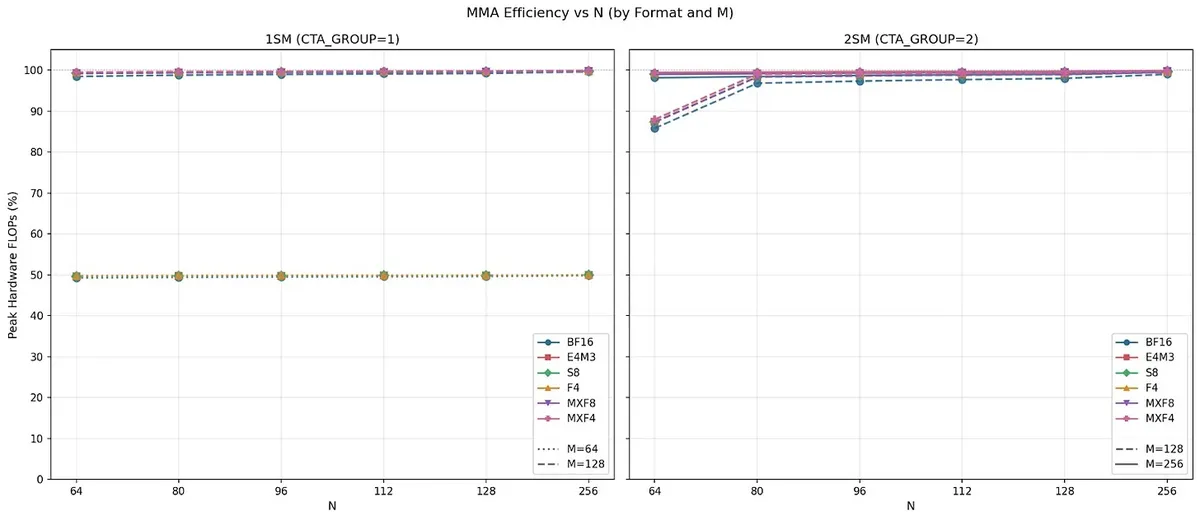

This connects nicely back to the TK abstractions we already introduced. At warp level, the natural objects were often vectors, and the natural operations were things like maps and reductions. For tensor-core compute, the natural objects are tiles, and the operation is matrix multiply-accumulate over those tiles.

The important detail is that the output tile is still not owned by one thread. On Hopper, an operation such as m64n64k16 produces a 64×64 accumulator tile, but that tile is distributed across the warpgroup. Each thread owns only its register fragment of the larger logical accumulator. So the rt abstraction is doing real work here: it lets us talk about the accumulator as one tile, even though physically it is spread across many lanes.

That is why, instead of writing raw wgmma.mma_async... PTX ourselves, we work with TK objects and call a wrapper such as:

warpgroup::mma_AB(C_accum, As, Bs);
warpgroup::mma_async_wait();

Here C_accum is the register tile accumulator, while As and Bs are the operand tiles. Conceptually, the warpgroup repeatedly updates the same accumulator tile from successive slices along the shared K dimension. The operands have already been staged into shared memory, and each MMA step consumes one K slice and accumulates into the same register-resident output tile.

On Blackwell, the same tile level story continues, but the accumulator storage changes. Instead of accumulating directly into register tiles, tcgen05 accumulates into tensor memory, which TK represents with tensor memory tiles such as tt<float, 128, 128>. So the high-level shape of the code still looks like “multiply these tiles and accumulate into this output tile,” but the output tile may now live in a different hardware storage space. We will come back to tensor memory in the next section!

There is a related input-side asymmetry worth keeping in mind too. On Hopper WGMMA, matrix A can come either from registers or SMEM, while matrix B must come from SMEM. On Blackwell tcgen05, the analogous choice is that matrix A can come from SMEM or tensor memory (TMEM), while matrix B still comes from SMEM This SS vs TS distinction matters because it changes how much pressure the MMA instruction puts on SMEM. In SS, both A and B are read from SMEM. In TS, A comes from TMEM while B still comes from SMEM. For M=128, TS reaches near peak throughput across the tested N sizes, while SS underperforms for smaller N and only catches up around N=128.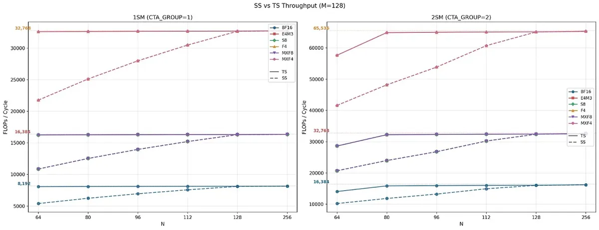



The reason is that small-N SS instructions can be SMEM bandwidth bound. For example, with an FP16 128×64×16 MMA, the instruction does not have enough math per byte of SMEM operand traffic yet, so feeding both A and B from SMEM takes more cycles than the tensor-core math itself. As N grows, the arithmetic intensity improves, and by N=128 the math side catches up.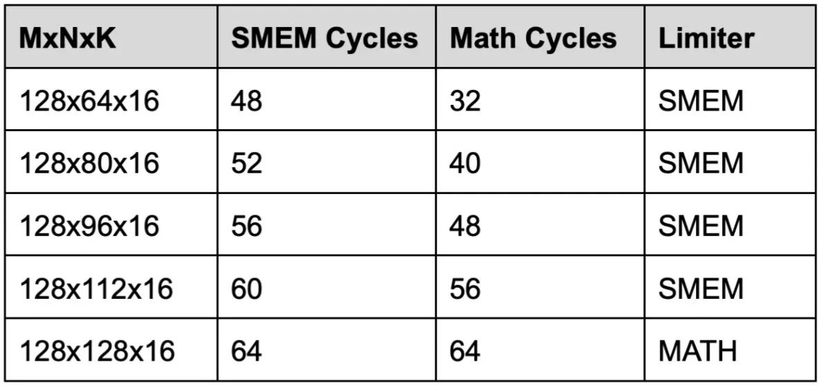



The roofline view says the same thing visually: smaller N points sit on the SMEM-bandwidth slope, while larger N reaches the flat compute-limited region.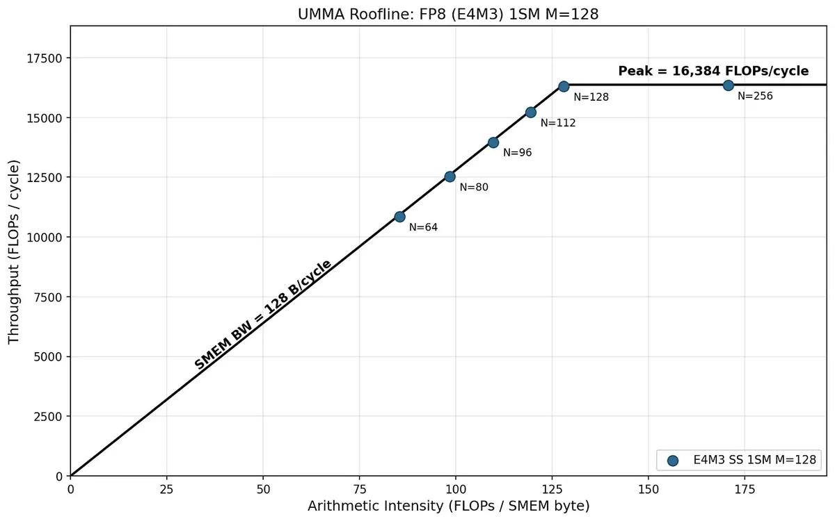



So TMEM is not only interesting because Blackwell accumulates into it. In the TS layout, using TMEM for A can also reduce pressure on SMEM and make the MMA easier to feed. .

One important detail is that Hopper wgmma is asynchronous. A warp-level add or sum feels like a direct collective operation. wgmma is different in the sense that the warpgroup issues one or more MMA instructions, commits them as a group, and later waits for the result.

That is why the TK call pattern has both the MMA call and an explicit wait:

warpgroup::mma_AB(C_accum, As, Bs);
warpgroup::mma_async_wait();

Inside warpgroup::mma_AB(...), TK fences the accumulator state, issues the underlying WGMMA calls across the needed K chunks, and then commits the group:

if constexpr (fence) { mma_fence(d); }
...
mma_commit_group();

So from our side, we still write tile level code, but underneath that call TK is coordinating an asynchronous tensor core operation.

There is one more hardware facing layer worth keeping in mind. Tensor core instructions do not consume SMEM like an ordinary instruction would. When an operand lives in SMEM, the tensor core needs a compact descriptor that tells it where the tile starts and how that tile is laid out.

This is exactly the kind of detail TK tries to hide from us. Whenever we write code using TK, we keep thinking in terms of st, rt, and, on Blackwell, tt objects. Underneath, TK turns the shared tile metadata into the descriptor values that the hardware instruction actually expects.

Conceptually, the tensor core needs answers to a few separate questions:

• Where are the SMEM operands, and how are they laid out?
• What MMA operation are we issuing?
• Do we want any special masking behaviour, such as treating some columns of B as zero? (Advanced option - will ignore this).

On Hopper, the first question is answered by the WGMMA matrix descriptor. This is a 64-bit value held in a register, and it describes the SMEM layout of an operand tile: its start address, leading dimension, stride dimension, and swizzle mode (32B, 64B or 128B).

The second question, however, is mostly answered by the PTX instruction variant itself. For example, an instruction such as wgmma.mma_async.sync.aligned.m64n64k16.f32.bf16.bf16 already tells the hardware the MMA shape and datatypes. So on Hopper, the SMEM descriptor tells the tensor core how to find the operand tiles, while the instruction name itself carries much of the operation metadata.

Blackwell keeps the same basic idea, but reorganises the interface. For the tcgen05 family, the PTX docs describe three descriptor objects.

1. The first is the Shared Memory Descriptor. This plays a role similar to the Hopper matrix descriptor: it describes a SMEM operand tile. The exact bit layout is slightly different from Hopper, but the mental model is the same: this descriptor answers “where is this shared tile, and how should the tensor core interpret its layout?”

2. The second is the Instruction Descriptor. This is the important new one. It is a 32-bit value in registers that describes the MMA operation itself: the operand types, accumulator type, M and N dimensions, transpose flags, whether the operation is dense or sparse, and, for microscaling formats, scale-factor metadata, and more. So compared with Hopper, more of the operation metadata has moved out of the PTX instruction name and into a descriptor.

That does not mean the tcgen05 PTX instruction says nothing. We still choose instruction families such as .kind::f16, .kind::f8f6f4, or block-scaled variants, and we still choose whether the operation is .cta_group::1 or .cta_group::2. But the detailed shape/type configuration is now largely carried by the instruction descriptor rather than by having a separate PTX instruction for every shape.

3. The third object is the Zero-Column Mask Descriptor. This is an optional advanced feature that lets the MMA behave as if selected columns of the B matrix were zero, regardless of the values actually present in shared memory. It is worth noting that this is not a general elementwise mask like the causal mask in attention. It is specifically a column structured mask over B, so I will ignore it for the main mental model here since TK doesn't use it.

Memory Movement Abstractions

So far, we have talked about the objects TK gives us and the compute operations we can perform on them. But before any of those compute paths can run, data has to move through the GPU memory hierarchy in the right shape and at the right time.

Shared Memory Allocation

In TK, kernels often begin with one raw block wide dynamic SMEM buffer, usually declared as something like:

extern __shared__ alignment_dummy __shm[];

The important idea is that the kernel first receives a scratchpad. Only afterward do we decide how to partition that scratchpad into useful typed regions.

In raw CUDA, we would usually have to do this partitioning manually. We would take the base pointer, offset it by some number of bytes, cast it to the type we want, then repeat that for the next buffer. TK wraps that small but annoying piece of bookkeeping in shared_allocator.

So instead of manually computing the offset for every SMEM object, we create an allocator from the raw SMEM buffer and ask it for the next region. Something like this:

shared_allocator al((int*)&__shm[0]);

st_bf<64, 64> (&As)[2] = al.allocate<st_bf<64, 64>, 2>();
st_bf<64, 64> (&Bs)[2] = al.allocate<st_bf<64, 64>, 2>();

Conceptually, shared_allocator behaves like a bump allocator. It starts at the beginning of the dynamic SMEM buffer, returns the current region reinterpreted as the requested type, and then advances its internal pointer so the next allocation starts after it.

The allocator is mainly needed at allocation time, not lookup time. Once a region has been allocated and bound to a variable, the kernel uses that returned reference directly. The allocator only remains useful for carving out the next SMEM object.

A useful mental model is that TK separates raw SMEM storage from typed SMEM objects. The raw __shm buffer is just storage. The allocator turns that storage into meaningful objects like st or sv.

Alignment is an important part of this design. The next object cannot always start exactly where the previous one ended. Sometimes the allocator has to move the pointer forward so that the next object starts on a valid boundary for the hardware or instruction being used. The skipped bytes are just padding.

The allocator does not reorder old allocations. It preserves allocation order and simply advances forward through SMEM, inserting padding when alignment requires it. This keeps the implementation simple and matches how these kernels stage multiple buffers sequentially.

One detail I like is the way allocate handles shaped allocations. When we write something like al.allocate<T, 2, 4>(); , the idea is not merely “allocate eight Ts” in the abstract. It is “treat the next SMEM region as a typed 2×4 array of T.” Physically the storage is contiguous, but semantically TK wants us to think in structured objects rather than raw flat buffers.

This small abstraction is a good example of TK’s broader philosophy: do not force the programmer to repeatedly solve low-level layout and bookkeeping problems in raw CUDA when those problems can be wrapped in a lightweight reusable abstraction.

Tensor Memory Accelerator (TMA)

The Tensor Memory Accelerator (TMA) is a dedicated hardware unit introduced with Hopper and continued/extended in Blackwell for moving multi-dimensional tensors. Instead of each thread calculating addresses and loading individual elements, TMA can transfer a tensor tile asynchronously between global memory and shared memory. It supports both GMEM -> SMEM and SMEM -> GMEM.

One naming caveat before we go further: TMA is not the same thing as Blackwell's tensor memory. TMA is the copy engine. Tensor memory is the on-chip accumulator storage used by Blackwell tcgen05 instructions. The names are annoyingly close, but they refer to different hardware ideas. We will talk about tensor memory later.

There are multiple advantages that TMA provides.

1. The first advantage is that the TMA hardware calculates addresses for bulk affine memory accesses of the form addr = width * base + offset for many bases and offsets concurrently. It does this using Tensor Maps, created with the cuTensorMapEncodeTiled CUDA Driver API. These tensor maps are descriptors that tell the TMA hardware the global tensor layout, the tile or box being moved, and the SMEM layout expected on the other side. Of course, TK abstracts creating these tensor maps for us as well, which we will see in a second. I am just trying to give the full picture first.

Offloading this work to the TMA hardware saves space in the very precious register file, reducing register pressure, and also reduces the demand on arithmetic bandwidth from the CUDA cores. Another important detail is that TMA instructions (PTX: cp.async.bulk.tensor, SASS: UTMALDG) are usually issued by a single thread, even though the data movement is serving the whole warp or warpgroup From the same SemiAnalysis experiments as referenced before, they stress-tested the TMA hardware on Blackwell and identified a key hardware behaviour. Their plot compares bytes-in-flight per SM against best-case TMA throughput.



In their benchmark, they used one CTA per SM with four warps, and had one elected thread from each warp issue TMA instructions over 2D tensor boxes ranging from 32×8 to 128×128. As bytes-in-flight increased, throughput initially rose sharply because there was now enough bulk copy work to amortise the setup cost. Once the curve flattens, the TMA path is saturated, so adding more bytes-in-flight does not buy much more throughput.

They also compare TMA against ordinary async copy. In SASS, ordinary async copy shows up as LDGSTS, while TMA shows up as UTMALDG. At small bytes-in-flight, ordinary async copy is slightly ahead, but as outstanding copy work grows, TMA catches up and scales to very high bandwidth.



The latency plot shows a different angle of the comparison. TMA can deliver high throughput, but individual TMA requests are not necessarily low latency, especially once the engine is heavily loaded.

.

2. The second advantage comes from TMA being asynchronous. Issuing the copy and consuming the result are separate events. This opened up a very natural memory/compute pipelining style, especially warp-specialised producer-consumer kernels, where producer warps launch memory movement while consumer warps keep the tensor cores busy on data that has already arrived. We will see what this paradigm looks like in more detail in the pipeline templates section.

TK hides almost all of the Tensor Map descriptor work from us. In raw CUDA, the lower-level picture is that a CUtensorMap descriptor has to be created on the host using cuTensorMapEncodeTiled(...), and then made available to the device so that the TMA instruction knows how to interpret the global tensor and the SMEM tile.

In TK, this happens as part of the gl abstraction. When we define something like:

using qo_tile   = st_bf<64, D>;
using qo_global = gl<bf16, -1, -1, -1, D, qo_tile>;

We are not just saying “this is a bf16 global tensor.” We are also telling TK, this global tensor may be moved with TMA using SMEM tiles of shape qo_tile.

So when the gl object is created, TK builds the corresponding CUtensorMap internally for that tile type. As users, we do not manually call cuTensorMapEncodeTiled(...), manually manage the descriptor, or pass raw tensormap pointers around.

Then inside the kernel, the surface we actually write is much smaller:

warp::tma::expect(...);
warp::tma::load_async(...);

For GMEM -> SMEM loads. If we want the reverse direction, SMEM -> GMEM, TK also gives us:

warp::tma::store_async(...);

One small detail worth keeping in mind is that warp::tma::... and warpgroup::tma::... are scope-level wrappers around the lower-level kittens::tma::... functions. The actual TMA instruction is issued down in the thread-level path. The warp or warpgroup wrapper is mainly telling us the intended scope of the operation.

Internally, these wrappers typically gate on laneid() == 0, because a TMA instruction only needs to be issued by one lane. So in principle, we could manually write something like:

if (laneid() == 0) {
    kittens::tma::load_async(...);
}

But the wrapper style is cleaner and safer. It encodes intent i.e this is a warp-scoped or warpgroup-scoped TMA issue, even if only one lane actually launches the instruction. So the mental model we need is that gl carries the global layout plus the TMA metadata, while warp::tma::load_async(...) is the device side operation that uses that metadata to move a tile into shared memory.

Moving into the more advanced features, starting from Hopper, SMs can be grouped through Thread Block Clusters. In CUDA, the portable maximum cluster size is 8 CTAs / thread blocks. H100 and Blackwell B200 can also support a cluster size of 16 CTAs, but only with an explicit non-portable opt-in.

CTAs in a Thread Block Cluster can communicate through Distributed Shared Memory (DSMEM). More precisely, DSMEM is a cluster-scoped shared-memory address space built over the separate shared-memory allocations of all CTAs in the cluster. Each CTA still has its own per-block SMEM allocation, but threads in the cluster can access the SMEM belonging to other CTAs in that same cluster. So the total DSMEM capacity is essentially:

Where:

• ${\text{DSMEM}}_{\text{cluster capacity}}$ is the total Distributed Shared Memory capacity available across the thread block cluster.
• $N_{\text{CTAs in cluster}}$ is the number of CTAs, or thread blocks, in the cluster.
• $SME{M}_{\text{shared memory per CTA}}$ is the shared-memory allocation for each individual CTA.

With Thread Block Clusters, Hopper TMA also supports multicasting. In multicast mode, a TMA load can transfer data from GMEM into the SMEM of multiple CTAs in the same cluster, with the destination CTAs selected by a multicast mask. Instead of each CTA independently issuing a GMEM load for the same operand tile, one TMA multicast operation can deliver that data to multiple CTA SMEM destinations.

In GEMM, this is useful because neighbouring CTAs often reuse the same operand tile. A multicast strategy lets CTAs split the operand load between members of a reuse group. Each CTA loads one slice, and TMA multicasts that slice into all CTAs that need it. After all slices arrive, each participating CTA has the full operand tile in its own SMEM. So multicast reduces redundant GMEM -> SMEM traffic, which can reduce L2 traffic Multicasting exhibits an interesting behaviour: Even when CTAs in a cluster issue ordinary TMA loads to the same global data, the hardware can coalesce some of those duplicate requests, giving something that looks like implicit multicast. It is not quite as clean as an explicit multicast TMA instruction, but it still reduces L2 traffic significantly compared with the case where each CTA loads completely different data.

The experiment compares three cases: a baseline where each SM loads different data, explicit multicast where one CTA issues a multicast TMA load to the CTAs in its cluster, and an implicit case where multiple CTAs issue ordinary TMA loads to the same global data.



The top plot reports SMEM fill throughput. With a cluster size of 2, explicit multicast can fill two CTAs' SMEMs from one shared data request, so the effective SMEM fill throughput is much higher than the baseline.

The bottom plot is the more revealing one: L2 bytes per SMEM byte. For the baseline, this is around 1.0. For explicit multicast with cluster size 2, it is around 0.5, which is the ideal 1 / cluster_size value. In other words, one byte fetched from L2 produces two bytes of SMEM fill across the cluster.

The implicit case performs similarly in SMEM fill throughput, but it leaks more L2 traffic as bytes-in-flight increases. So I guess the practical lesson is: if the sharing pattern is known, explicit TMA multicast is the cleaner and more reliable way to reduce L2/HBM traffic. and ultimately HBM traffic. Modular's Blackwell GEMM series explains this really well in Kernel 5, so I am going to adapt their visual here to make the idea concrete.

Blackwell then goes further with 2xSM MMA, exposed through tcgen05.mma.cta_group::2. TMA multicast can reduce redundant GMEM loads, but with ordinary single-CTA MMA, the same operand tile may still be duplicated across the shared memories of multiple CTAs because each CTA needs its own local copy for its own MMA.

Blackwell’s 2xSM MMA lets a pair of CTAs / SMs cooperate on one larger MMA operation. The two CTAs still produce separate output tiles, usually stacked along the M dimension, but the MMA instruction is aware of the CTA pair. That means an operand shared by the pair, such as the B tile in this picture, does not necessarily need to be fully duplicated in both CTAs’ shared memories. Each CTA can hold part of that operand, and the cta_group::2 instruction consumes the pair as one distributed operand.

So 2xSM MMA addresses a different bottleneck from multicast: not just redundant GMEM -> SMEM loading, but duplicated SMEM storage and operand movement into the tensor-core pipeline.

// From the TK B200 bf16 GEMM example, adapted to our drawing notation.
static_assert(_Mb == 256, "Mb must be 256"); // _Mb is the whole 2 CTA pair M tile.
static_assert(_Nb >= 16 && _Nb <= 256 && _Nb % 16 == 0, "Nb must be 16, 32, ..., 256");
static_assert(_Kb >= 16 && _Kb % 16 == 0, "Kb must be a multiple of 16");

// Drawing notation:
// BM    = per CTA M tile
// MMA_N = logical N tile of the MMA
// BK    = K tile
static constexpr int BM = _Mb / 2; // 128
static constexpr int MMA_N = _Nb;
static constexpr int BK = _Kb;

static constexpr int CLUSTER_SIZE = 2; // 2 CTA cluster
...
const int cta_rank = cluster_ctarank(); // 0 or 1
...
// The tile shapes expose the 2xSM structure:
//
// A pair           = 2BM × BK
// B pair           = MMA_N × BK
// Accumulator pair = 2BM × MMA_N
using a_tile = st_bf<BM, BK>; // Each CTA owns a full BM × BK A tile.
using b_tile = st_bf<MMA_N / 2, BK>; // Each CTA owns only half of the B tile.
using d_tt_t = tt<float, BM, MMA_N>; // Each CTA accumulates BM × MMA_N in TMEM.

We can see this being used in TK's bf16 B200 GEMM kernel. The tile shapes in the kernel line up directly with our 2xSM MMA visual. TK’s _Mb represents the M dimension of the whole 2-CTA pair, so the per-CTA M tile is _Mb / 2. Each CTA therefore owns a full BM × BK A tile for its own output rows.

The B tile is different. Each CTA stores only MMA_N / 2 × BK, while the accumulator for each CTA still spans BM × MMA_N. This is the key 2xSM pattern: B stays distributed across the pair, but the MMA instruction consumes both halves as one logical B operand.

In TK, the multicast-capable path for TMA is exposed through tma::cluster::load_async, and it takes the following arguments:

tma::cluster::load_async(
    smem_tile, // destination shared tile
    global_tensor, // global layout descriptor
    tile_coord, // tile coordinate in the global tensor
    semaphore, // semaphore / mbarrier used for async completion
    cluster_mask, // which CTAs receive the TMA load
    dst_mbar_cta // which CTA owns the mbarrier to signal, default -1
);

In the B200 GEMM example, the B load looks like this:

tma::cluster::load_async(
    b_smem[input_ring],
    g.b,
    {tile_coord.y * 2 + cta_rank, idx},
    inputs_arrived[input_ring],
    (uint16_t)(1 << cta_rank),
    0
);

Here the mask is 1 << cta_rank, so each CTA loads into its own SMEM only. CTA 0 loads one B half, CTA 1 loads the other B half, because again we are setting up a 2xSM MMA rather than duplicating the full B tile in both CTAs.

The last 0 means the completion is signaled to CTA 0’s mbarrier. So both CTAs issue their own loads, but CTA 0 waits until the distributed operand pieces are ready, then issues the 2-CTA MMA.

else if (cta_rank == 0 && warpgroup::warpid() < C::NUM_CONSUMERS && warp::elect_leader()) {
    ...

    for (int idx = 0; idx < iters_per_task; idx++) {
        if (idx == 0)
            mm2_ABt(...); // first K slice: initialise D = A @ B
        else
            mma2_ABt(...); // later K slices: accumulate D += A @ B
    }

    ...
}

The 2 in mm2_ABt / mma2_ABt is the TK abstraction for the tcgen05.mma.cta_group::2 PTX instruction.

Tensor Memory

On Hopper, wgmma accumulates into registers, so the output tile is represented naturally as a register tile, rt. What that also means, however, is that the accumulator competes with the rest of the kernel for register space. In kernels with deep pipelines, those registers are precious.

Blackwell changes this by adding a new storage space called tensor memory (TMEM). It is still on chip storage inside each Streaming Multiprocessor (SM), but it is dedicated to tensor core instructions rather than being ordinary per thread register storage. The useful mental model is that tensor memory gives the tensor cores their own accumulator space.

So instead of every accumulator fragment living in the general register file, tcgen05.mma can accumulate into tensor memory. TK represents that storage with tensor memory tiles such as tt<float, 128, 128>.

That changes the MMA dataflow across recent architectures as follows:

On older tensor core paths, the accumulator naturally flows back into register memory. On Blackwell, tcgen05.mma writes the accumulator into TMEM instead. Matrix A can come from SMEM or TMEM, matrix B comes from SMEM, and the output D lands in TMEM. Later, if the kernel needs to run an epilogue or write the result back to global memory, it explicitly moves data out of TMEM again. This opens up new opportunities for pipelining strategies that overlap memory loads, stores and tensor core compute compared with older architectures. We will look into this more in a future section when we talk about scheduling, so let's save that for later!

Physically, TMEM is a 256KB on chip memory space per SM. It is structured as a 2D array of 128 lanes and 512 columns, with each cell holding 32 bits, or 4 bytes. So the full capacity is:

Allocation happens by columns, with a granularity of 32 columns. That means the smallest allocation is:

at a time.

There are two separate ideas in this layout.

The first is allocation. TMEM is allocated dynamically using tcgen05.alloc, and allocation happens in units of columns. When a column is allocated, all 128 lanes of that column are allocated together. The number of columns allocated must be a power of two and at least 32, which matches the 32 column minimum allocation we showed above. TMEM also has to be explicitly deallocated with tcgen05.dealloc.

For cta_group::1, tcgen05.alloc and tcgen05.dealloc are issued by a single warp, and the same warp should both allocate and deallocate the TMEM region. For cta_group::2, the allocation is collective across the CTA pair, so one warp from each peer CTA participates. One slightly unintuitive detail is that tcgen05.alloc stores the base 32 bit address of the allocation into SMEM. That TMEM base address is then used as the offset to the accumulator tensor for the UMMA instruction.

tcgen05.alloc is also a blocking instruction. If the requested TMEM columns are not currently available, the issuing warp can block until enough TMEM becomes free. So TMEM allocation is a runtime resource management operation.

There is also a tcgen05.relinquish_alloc_permit instruction, which tells the hardware that this CTA will not perform any more TMEM allocations. After a CTA relinquishes this permit, issuing another tcgen05.alloc from that CTA is illegal. So tcgen05.alloc asks the hardware for some TMEM columns, tcgen05.dealloc returns a specific TMEM allocation, and tcgen05.relinquish_alloc_permit tells the hardware that this CTA is done allocating TMEM.

The second idea is access. TMEM is not freely accessed like SMEM. It has a restricted access pattern. For tcgen05.ld and tcgen05.st, one warp can only access its own 32 lane slice of TMEM, so it takes a full warpgroup to cover all 128 lanes.

Typically, data gets into TMEM through UMMA operations themselves, and is moved out to registers using tcgen05.ld for post processing. It is also possible to manually move data into TMEM: tcgen05.cp can copy from SMEM into TMEM, and tcgen05.st can store from registers into TMEM. But these paths are much more restricted than ordinary loads and stores. The movement instructions operate on fixed data movement shapes, while the MMA instruction writes D into hardware-defined TMEM datapath layouts.

Let's go one level deeper into the movement side and understand these shapes, as we did earlier in the blog for register fragment layouts. The following shapes are the ones supported by tcgen05.ld, tcgen05.st, and tcgen05.cp:

Let's look at tcgen05.ld, which is used to copy data from TMEM to RMEM. Since the loads are warp-level instructions, let's zoom into warp 0 and specifically the tcgen05.ld.sync.aligned.shape.num.b32 instruction to see what the load of this warp will look like from TMEM to RMEM. There are various other shapes which are all documented here, but this will suffice to understand the idea.

tcgen05.ld.sync.aligned.shape.num.b32 r, [taddr];

.shape = { .16x64b, .16x128b, .16x256b, .32x32b }
.num   = { .x1, .x2, .x4, .x8, .x16, .x32, .x64, .x128 }

The key thing to notice is that 32x32b is not a 32×32 matrix tile. It means: access 32 TMEM lanes, and read 32 bits from each lane. The .num modifier then repeats that access along the column direction.

So for:

tcgen05.ld.sync.aligned.32x32b.x1.b32 r, [taddr];

one warp reads:

Each of the 32 threads receives one 32 bit register. If we instead use .x2, the same 32 lane load is repeated across two columns, so each thread receives two 32 bit registers. With .x4, each thread receives four registers, and so on.

This also explains the warpgroup restriction more concretely. Warp 0 can access lanes 0..31, warp 1 can access lanes 32..63, warp 2 can access lanes 64..95, and warp 3 can access lanes 96..127. So a single warp can move a 32 lane slice, but touching the full 128 lane height of a TMEM tile requires the whole warpgroup.

tcgen05.st follows the same kind of logic in the opposite direction, moving data from registers into TMEM. tcgen05.cp is a different path, moving data from SMEM into TMEM.

The .32x32b example above is useful as a simple mental model, but TK does not expose the whole PTX shape menu directly to us. Instead, its wrappers choose particular movement shapes based on the tile dtype and register tile layout. For eg. 16-bit values such as bf16 and half, uses tcgen05.ld.sync.aligned.16x128b.x2.pack::16b.b32 in TK:

This is the same basic idea as above, but with a different shape. The instruction touches 16 TMEM lanes, reads 128 bits per lane, and repeats that access twice in the column direction. Because of pack::16b, each 32-bit destination register contains two 16-bit values packed together. So each thread receives four 32-bit registers, carrying eight 16-bit values. The important design point is not the exact shape itself, but that TK hides this PTX shape selection behind typed operations such as warpgroup::load_async.

Let's now tie this back to how TK approaches handling this new hardware. Firstly, the tile abstraction for tensor memory is provided as tt<T, rows, cols>:

template<typename _T, int _rows, int _cols>
struct tt {
    using identifier = ducks::tt::identifier;

    using T = base_types::packing<_T>::unpacked_type; // scalar type
    using T2 = base_types::packing<_T>::packed_type; // vector type (e.g. bf16_2)
    using dtype = T;

    static constexpr int rows = _rows;
    static constexpr int cols = _cols;

    static_assert(rows / (4 / sizeof(T)) <= MAX_TENSOR_ROWS, "Row dimension must be less than or equal to MAX_TENSOR_ROWS");
    static_assert(cols / (4 / sizeof(T)) <= MAX_TENSOR_COLS, "Column dimension must be less than or equal to MAX_TENSOR_COLS");
    static_assert(rows % kittens::BASE_TILE_DIM == 0, "Row dimension must be divisible by the 16");
    static_assert(cols % kittens::BASE_TILE_DIM == 0, "Column dimension must be divisible by the 16");

    uint32_t addr; // The only runtime data: Tensor Memory address handle
    ...
};

// Notice at the top there are these constants ensuring the requested row and column dimensions
// never exceed the underlying TMEM layout, matching the structure in our drawing.
constexpr int MAX_TENSOR_ROWS = 128; // TMEM lanes
constexpr int MAX_TENSOR_COLS = 512; // TMEM columns

_T is the element type we ask for, for example bf16, float, or fp8e4m3. We do not manually pass the packed register/container version ourselves. Instead, TK normalizes the type through base_types::packing. For every type TK supports, base_types::packing defines both an unpacked type and a packed type. So if we write tt<bf16, 128, 128>, then T is bf16 and T2 is bf16_2.

Again, tensor tiles need to be divisible by 16 across both the row and column dimensions. This matches the rest of the DSL's building-block narrative: TK likes to organize work around 16-wide base tiles. The other important check is that the requested tile must fit inside the physical TMEM layout we drew earlier: 128 lanes by 512 columns.

One subtle detail in the asserts is this:

rows / (4 / sizeof(T))
cols / (4 / sizeof(T))

// Each cell in the TMEM layout is a 32-bit cell, i.e. 4 bytes, so:
//
// 4 / sizeof(float) = 1
// 4 / sizeof(bf16)  = 2
// 4 / sizeof(fp8)   = 4
//
// In other words, this tells us how many logical T values fit inside one
// 32-bit TMEM cell:
//
// float: one logical element per 32-bit TMEM cell
// bf16:  two logical elements per 32-bit TMEM cell
// fp8:   four logical elements per 32-bit TMEM cell

TMEM is not normal C++ memory. As we said earlier, we do not access it through ordinary loads and stores. We access it through instructions like tcgen05.mma, tcgen05.ld, tcgen05.st, and tcgen05.cp. That is why the tt object does not store the tile data itself. It stores only a 32-bit TMEM address handle:

uint32_t addr;

The address points to the top left coordinate of the tensor tile view. In other words, tt<float, 128, 128> is not “128 by 128 floats stored inside the C++ object.” It is a typed view over a 128 by 128 region of TMEM, starting at addr.

The initial tile address ultimately comes from tensor_allocator, which calls tcgen05.alloc. TK can also create smaller TMEM views from a larger one using subtile:

template<ducks::tt::all TT>
__device__ inline TT subtile(int row_offset, int col_offset) const {
    return TT(
        addr
        + (row_offset << 16)
        + col_offset / (4 / (uint32_t)sizeof(T))
    );
}

This is one of the nicest parts of the abstraction. A subtile does not copy data. It just returns a new tt object with a different TMEM address. The new address points to a different top left coordinate inside the same underlying TMEM allocation.

For tt<float, 128, 128>, the math is especially clean because sizeof(float) = 4, so each logical float occupies exactly one 32-bit TMEM cell. That means logical columns and physical TMEM columns line up one-to-one. The subtile formula therefore just moves down by shifting the row offset into the lane bits, and moves right by adding the column offset.

The high 16 bits of the address encode the lane coordinate, and the low 16 bits encode the column coordinate. Let's look at an example of how this would look, adapting the TMEM layout drawing from above:

We hinted earlier that the initial tile address comes from tensor_allocator, which is the abstraction that wraps the actual tcgen05.alloc PTX instruction and communicates with the hardware. A tt object can point to a typed tile view inside TMEM, and it can create smaller subtile views from that tile, but it does not provision or deprovision TMEM itself. For that, TK uses tensor_allocator.

template<int _nblocks_per_sm, int _ncta, bool _managed = true>
struct tensor_allocator {
    static constexpr int nblocks_per_sm = _nblocks_per_sm;
    static constexpr int cols = ((MAX_TENSOR_COLS / nblocks_per_sm) / 32) * 32;
    static constexpr int ncta = _ncta;
    static constexpr bool managed = _managed;

    uint32_t addr;
    ...
};

// _nblocks_per_sm:
// tensor_allocator<1, ...>
//   cols = 512
//   one block per SM gets the full 512 TMEM columns

// tensor_allocator<2, ...>
//   cols = 256
//   two blocks per SM each budget 256 TMEM columns

The first template parameter, _nblocks_per_sm, is a capacity-budgeting parameter. It tells TK how much of the SM's TMEM column space this allocator should reserve. It does not mean the allocator knows what tile shapes we will create later. Instead, it decides the total TMEM budget up front.

For example, if we construct:

tensor_allocator<1, 1> tm_alloc{};

then because _managed = true by default, the constructor provisions TMEM for us. Since _nblocks_per_sm = 1, TK computes:

So this managed allocator provisions 512 physical TMEM columns across all 128 lanes. In other words, it reserves the full TMEM column budget represented by this allocator.

The actual hardware allocation is wrapped in provision:

__device__ inline void provision(uint32_t &shared_addr) {
    if constexpr (ncta == 1) {
        asm volatile(
            "tcgen05.alloc.cta_group::1.sync.aligned.shared::cta.b32 [%0], %1;\n"
        ::  "l"(reinterpret_cast<uint64_t>(&shared_addr)), "n"(cols)
        );
        asm volatile("tcgen05.relinquish_alloc_permit.cta_group::1.sync.aligned;\n");
    }
    else {
        asm volatile(
            "tcgen05.alloc.cta_group::2.sync.aligned.shared::cta.b32 [%0], %1;\n"
        ::  "l"(reinterpret_cast<uint64_t>(&shared_addr)), "n"(cols)
        );
        asm volatile("tcgen05.relinquish_alloc_permit.cta_group::2.sync.aligned;\n");
    }
}

This matches the PTX detail we saw earlier: tcgen05.alloc does not return the TMEM address like a normal C++ function. Instead, it writes the allocated TMEM base address into shared memory. That is why provision takes shared_addr by reference. After allocation, TK immediately calls tcgen05.relinquish_alloc_permit, which tells the hardware that this CTA will not request more TMEM allocations.

When _managed = true, the constructor calls provision automatically:

__device__ inline tensor_allocator() {
    if constexpr (managed) {
        __shared__ uint32_t shared_addr;
        if (warpid() == 0) provision(shared_addr);
        asm volatile("tcgen05.fence::before_thread_sync;\n");
        asm volatile("bar.sync 0;\n");
        asm volatile("tcgen05.fence::after_thread_sync;\n");
        set_addr(shared_addr);
    }
}

Only warp 0 performs the allocation, because tcgen05.alloc is issued by a warp. The barriers and TMEM fences make sure the allocated address is ready before the rest of the CTA starts creating tt views from it.

Later, if we do:

tm_alloc.template allocate<tt<float, 128, 128>>(0);

TK creates a tt<float, 128, 128> view covering lanes 0..127 and columns 0..127. If we create another view:

tm_alloc.template allocate<tt<float, 128, 128>>(128);

then that view covers lanes 0..127 and columns 128..255.

This is a key design point:

The allocator does not size itself based on future tile requests. Instead, it reserves the whole budget up front based on the number of blocks expected to use the same SM.

The second template parameter, _ncta, controls the CTA-group mode used by the underlying PTX instruction. If _ncta=1, TK emits tcgen05.alloc.cta_group::1. If _ncta=2, TK emits tcgen05.alloc.cta_group::2, meaning the allocation and deallocation are collective across a CTA pair. As we said earlier, for cta_group::2, one warp from each peer CTA participates. I hope I explained the bigger picture of TMEM clearly. Now, let’s look at the pipeline templates that ThunderKittens provides, which are the highest level of abstraction in TK for writing kernels quickly.

Pipeline Templates

Up to this point, most of what we have looked at in TK has been about what objects exist and what operations we can perform on them. Pipeline templates are where those abstractions start to get assembled into something closer to a full kernel skeleton.

This is an important point, because TK really operates at two different layers.

At the lower layer, TK gives us the core building blocks: gl, st, rt, sv, rv, together with the compute and memory abstractions built on top of them. Those abstractions are useful even if we end up writing a fairly hand-rolled kernel ourselves. At an even higher layer, TK also provides prototype pipeline templates such as lcf and lcsf, which package a common execution pattern into reusable scaffolding.

So if a kernel fits one of these prototype templates, TK can give us much more than just nice tile abstractions. It can also give us a ready-made pipeline structure. If a kernel does not fit the prototype layer cleanly, that still does not mean TK stops being useful. It simply means we fall back to using the lower abstraction layer directly.

A good way to think about the prototype system is as a small stack of layers:

• a kernel schema
• a pipeline hook interface
• a pipeline engine

The first of these, the kernel schema, is template-agnostic. In the common prototype layer, TK defines a minimal kittens_layout concept. At the most basic level, a pipelined kernel must provide globals and an input_block. In other words, the user-defined layout tells TK what the kernel operates on and what unit of data is going to flow through the pipeline.

That minimal schema is then normalised through complete_kittens_layout. This is where optional pieces such as scratch_block, finish_block, producer_state, consumer_state, and output_block are filled in with defaults like empty if they are not explicitly provided. Conceptually, this step matters because it lets the generic engine compile against one uniform internal schema, instead of constantly branching on whether a given layout happened to define every optional type.

Once that schema exists, each pipeline template defines its own hook interface. This is what the templates.cuh files are really doing. They are not the execution engine itself. Rather, they define the argument bundles that get passed into the different hook functions such as common_setup, producer::load, or consumer::compute.

The key idea is that every hook gets a shared base context through uniform_args, and then each stage-specific argument pack inherits from that base and adds only the extra data needed for that phase. So conceptually, the hook interface separates:

• the data every stage always needs
• the data only a particular stage needs

That is a small but important design choice. It means the template interface is not one giant, monolithic kernel argument struct. Instead, the structure of the arguments mirrors the structure of the pipeline itself.

A useful mental model is:

• setup hooks initialise per-role state before the main iteration loop
• load hooks fill one pipeline slot for a specific iteration
• compute hooks consume one pipeline slot for a specific iteration
• finish hooks perform per-task finalisation after all iterations are done

This also explains why the hook arguments differ. producer::setup does not need an input tile, because it is not loading any particular stage yet. It is only preparing the producer side of the kernel, for example by adjusting register allocation or initialising producer-local state. By contrast, producer::load is the phase that fills a concrete pipeline slot, so it needs the current input block, the current iteration index, and the synchronisation object used to signal that the slot is ready.

The same logic appears on the consumer side. consumer::setup is for one-time initialisation for the current task, while consumer::compute is the per-iteration phase and therefore needs the current pipeline slot and iteration-specific context.

At this point we can see what the prototype templates are really buying us. They are not writing the math for us. We still define the actual kernel-specific work in these hooks. But they do package the repetitive orchestration: the role split, the shared-memory staging structure, and the synchronisation pattern.

That brings us to the pipeline engines themselves.

The simplest one to look at is lcf, which stands for load-compute-finish. The idea is exactly what the name suggests. Data is loaded into staged shared-memory slots, consumed by the compute phase, and then a final epilogue or writeback-style phase runs once all iterations for that task are complete.

lcsf extends the same basic idea into load-compute-store-finish. The important difference is that lcsf introduces a distinct output-stage path, so storing is no longer folded into the final epilogue alone. That is why its hook interface includes an extra producer-side store hook.

At a high level, then, lcf and lcsf share the same overall philosophy, but lcsf makes the output path more explicit. In practice, that makes sense for kernels where output staging is itself substantial enough to deserve its own pipeline role.

Another useful way to think about these templates is as a producer-consumer ring-buffer pattern over shared-memory stages. The deep idea is not really the name of the primitive being used for synchronisation. The deep idea is the reusable-slot handoff protocol:

• producer marks a slot ready
• consumer uses that slot
• consumer marks it free
• producer reuses it

That pattern should look familiar if you have ever written a warp-specialised CUDA kernel by hand. In fact, this is exactly the same high-level producer-consumer structure I used in my own H100 GEMM worklog. There, I happened to express the handoff with full and empty barriers. In TK, the same conceptual handoff is expressed with semaphores such as inputs_arrived and inputs_finished. The specific synchronisation abstraction differs, but the underlying pipeline idea is the same.

So when reading TK’s names, it helps to think semantically rather than syntactically:

• inputs_arrived means the slot is ready for consumers
• inputs_finished means the slot is free for producers to reuse

In other words, a ring buffer is the scheduling pattern, while the barriers or semaphores are just the mechanism used to implement the handoff.

Stepping back, the main value of these prototype templates is not that they magically replace kernel design. We still need to decide what the task is, what lives in shared memory, what lives in registers, how many iterations a task requires, and what work belongs in setup versus compute versus finish. But for kernels that fit this staged structure well, the templates save us from repeatedly rewriting the same orchestration logic around those decisions.

It is also worth saying explicitly that not every kernel fits neatly into this prototype layer. A GEMM-style or attention-style kernel often maps onto these templates very naturally. Something like LayerNorm or RMSNorm may align more strongly with the lower abstraction layer than with the full prototype scaffolding. But that is not a weakness of TK. It is just a reminder that the real value of the framework is broader than the prototype layer alone.

So the right question is not simply, “does this kernel use a TK prototype template?” The more important question is whether TK’s abstractions still make the kernel easier to reason about and implement. Quite often, even when the answer at the prototype level is no, the answer at the abstraction level is still very much yes.

For completeness, another prototype that appears in the codebase is lcsc, which is aimed at more communication-heavy parallel kernels. That becomes especially relevant for distributed or multi-GPU settings, which are out of scope for this post. Here, I mainly want to focus on the load-compute style templates because they are the ones most directly relevant to the attention kernels we are about to build.

To make that a bit more concrete, it helps to finally look at what the lcf engine is actually doing in the source.

The first thing it defines is a kernel_template concept. This is simply the contract that a kernel template parameter must satisfy. In practice, that means the type must provide a layout, a producer, a consumer, and the expected hook functions such as common_setup, producer::setup, producer::load, consumer::setup, consumer::compute, and consumer::finish. The layout itself must still satisfy kittens_layout, so the engine can rely on at least globals and input_block being present.

One useful detail here is that the shared-memory budgeting is done entirely in bytes. So when the code uses values such as 1024, that means 1024 bytes = 1 KiB. Likewise, MAX_SHARED_MEMORY = 227 * 1024 should be read as roughly 227 KiB of shared-memory budget per block on Hopper.

// include/common/util.cuh
#if defined(KITTENS_HOPPER) || defined(KITTENS_BLACKWELL)
constexpr int MAX_SHARED_MEMORY = 227 * 1024;
#endif

// prototype/common/templates.cuh
FLAG_GETTER(MAX_SHARED_MEMORY, ((kittens::MAX_SHARED_MEMORY/NUM_BLOCKS_v<T>)-512))

The intuition is that Hopper exposes a 256 KiB combined L1/SMEM pool, with a configurable shared-memory carveout of roughly 228 KiB, and then about 1 KiB per block is still reserved for system use. So these constants are really shared-memory budgeting policies, not thread-related quantities.

The producer-consumer role split inside lcf is also static rather than dynamic. The block already contains all the warps it is going to use, and the engine assigns their role according to warp id. With the default lcf configuration, NUM_CONSUMER_WARPS = 8 and NUM_PRODUCER_WARPS = 4, which corresponds to two consumer warpgroups and one producer warpgroup. The per-stage handoff objects inputs_arrived[i] and inputs_finished[i] belong to the input-stage ring itself, while finish_finished protects the separate finish phase.

We can also see thatlcf supports persistent-kernel launches with the outer loop over task_iter. One block is not simply launched for one tile and then finished. Instead, the same block keeps pulling logical tasks from a persistent task stream until common_setup(...) indicates that there is no more work to do. It is useful here to distinguish two levels of looping:

• task_iter tells us which logical task this persistent block is currently working on
• num_iters tells us how many inner streamed iterations that one task requires

I am used to GEMM so a good analogy that made it easier to visualise, is that one task_iter might correspond to one output tile of C, while num_iters would be the number of K-slices that need to be streamed through the pipeline to accumulate that tile. We will get to persistent kernels in the next section when we talk about grid scheduling in more detail.

The actual per-stage reuse then happens through the input stage ring. Each SMEM stage is just one reusable slot. The producer waits until a slot has been marked reusable, fills that slot, and advances the ring index modulo the number of stages. The consumer waits until a slot has arrived, computes using that slot, and then marks it free again. That steady state handoff is the actual heartbeat of the pipeline.

One subtle but very important part of the lcf engine is that dynamic shared memory is partitioned according to lifetime, not just by simple forward allocation. scratch_smem holds per-task shared state that persists across the whole iteration loop. input_smem[stage] forms the ring of per-iteration input buffers. And finish_smem is a separate epilogue region used only at the end of the task.

The interesting part is that finish_smem is not allocated together with the forward input stage buffers. Instead, it is placed manually near the end of the SMEM budget. This lets the engine start preloading the next task into the early "safe" input stages while the previous task is still finishing, without immediately clobbering the still live finish region. In other words, the layout is not just about where data fits. It is about which regions can be safely reused at different moments in the persistent pipeline.

That is exactly what NON_FINISH_BLOCK_SPACE and SAFE_STAGES_BETWEEN_BLOCKS are quantifying. They tell the engine how much of the input stage ring can be reused safely before the producer must wait for finish_finished. So the point of this logic is not only alignment. It is safe SMEM packing across task boundaries in a persistent pipelined kernel.

So the real value of the prototype layer is not that it removes kernel design. It is that it packages the orchestration around kernel design. We still decide what the task is, what lives in SMEM, what lives in registers, and what work belongs in setup, compute, and finish. But when the kernel fits the staged structure well, TK saves us from rewriting the same role split, staging, and synchronisation machinery every time.

Tile Scheduling Strategies

Tiling is one of the most important optimisations on GPUs. The basic idea is that instead of treating the full computation as one huge chunk of work, we split it into smaller logical tiles. In the simplest case, each of these tiles can then be assigned to a CTA / thread block, so that the GPU can run many independent pieces of work in parallel across its (Streaming Multiprocessors) SMs.

But once we split the problem into tiles, another question appears: how do we actually schedule those tiles?

In this section, we will start from the most basic naive way of scheduling tiles, and then build towards more advanced strategies such as persistent kernels / persistent scheduling, and finally Blackwell’s Cluster Launch Control (CLC) scheduling. We will also look at a CTA traversal technique used in ThunderKittens called supergrouping, which is meant to improve L2 reuse by making nearby CTAs work on tiles with useful data locality.

We will follow a GEMM problem for this like we have done before:

where:

The computation of C is parallelised by dividing the problem shape (M, N, K) using tile sizes BM, BN, and BK. Each logical output tile C[i, j] has shape BM x BN, and is computed by accumulating over the tiled K dimension:

So C[i, j] is the work tile we care about in this section. The scheduling question is basically: which CTA, or CTA cluster, computes this tile, and when?

Single Tile Scheduling & The Wave Quantisation Problem

SMs on an NVIDIA GPU contain the compute units and can work independently of each other. On H100 SXM, we have 132 SMs, and on B200 we have 148. So an ideal workload should take maximal advantage of the parallelism between the SMs and distribute the work between them evenly, so that all the SMs are busy and none of them are sitting idle. Otherwise, that is just wasted compute capacity that we are leaving on the table. If some SMs finish their assigned work earlier than others, then they will sit idle until all the others have finished. This is called load imbalance.

Consider the following simplified example, which follows the most basic single tile scheduling strategy, where each BM x BN output tile is assigned to a CTA, and each CTA computes its assigned work on an available SM.

If we have this 4 x 4 tile grid, then we have 16 total output work tiles. Let's imagine we are on hypothetical hardware that has only 4 SMs. In that case, assuming one CTA occupies one SM, the kernel finishes the work in 4 full waves. Every wave has 4 CTAs running, so all 4 SMs are doing useful work throughout the execution.

In the other case, where our hypothetical hardware has 5 SMs, the first 15 tiles will be scheduled in 3 full waves. But the final 16th tile will be scheduled in a wave on its own. So even though we have more SMs, the final wave only has one useful CTA running, while the other 4 SMs are sitting idle. This is the wave quantisation problem.

Definition: In a GPU, a wave refers to a batch of CTAs / thread blocks that can be resident on the GPU at roughly the same time. The total number of waves is given by CEIL_DIV((M/BM) * (N/BN), num_SMs).

You can imagine this for a real H100 SXM with 132 SMs. Suppose we launch a kernel with 132 CTAs, and assume again that only one CTA can run per SM. In that case, the kernel finishes in a single full wave. But if we increase the launch to 133 CTAs, suddenly we need an extra wave. That second wave contains only one CTA, so almost the whole GPU is idle during that final part of the kernel.

This is why wave quantisation can be quite painful. The runtime does not always scale smoothly with the number of work tiles. Instead, it gets rounded up by the number of waves needed to finish all the CTAs. This effect is especially noticeable when the total number of work tiles is small, or when it is just slightly above a wave boundary.

Additionally, there are usually overheads associated with launching and tearing down CTAs. These arguments motivate the next scheduling strategy.

Static Persistent Tile Scheduling

In this strategy, instead of launching one CTA per output tile and letting each CTA exit after finishing one tile, we launch a fixed set of persistent workers, and each worker processes multiple tiles over time.

In the simplest case, the persistent worker is just one CTA. So if we have 4 SMs, we may launch 4 CTAs, assuming one persistent worker per SM for simplicity, and each CTA stays alive on the GPU, repeatedly walking through tiles from a fixed static sequence. Conceptually, CTA 0 handles tile 0, then tile 4, then tile 8, and so on. CTA 1 handles tile 1, then tile 5, then tile 9, etc. The stride is the number of persistent workers.

On Blackwell, especially when using 2xSM MMA, the persistent worker is often not a single CTA anymore. Instead, the worker is a CTA cluster. For example, with cluster size 2, each worker is a pair of CTAs cooperating together. So if we have 4 SMs and cluster size 2, we only have 2 persistent workers. Each worker is one cluster, and each cluster contains 2 CTAs.

So the scheduling arithmetic changes slightly. In the single CTA case, the stride is the number of CTAs. In the clustered case, the stride is the number of clusters. The CTAs inside a cluster do not independently choose different output tiles. They cooperate on the same scheduled tile, and cta_rank decides which part of the work each CTA performs inside that cluster.

This is the idea behind static persistent tile scheduling. The schedule is still static because the next tile is determined by simple arithmetic. But the kernel is persistent because the same worker stays alive and keeps moving through multiple "logical" tiles.

Compared to single tile scheduling, this gives us more control over how tiles are traversed. It also lets us amortise some of the fixed setup cost across multiple tiles, and gives the kernel a place to overlap work across tiles, such as overlapping one tile’s epilogue with another tile’s mainloop The tcgen05 for dummies post has a nice intra-kernel profiling example showing this effect. In the non-persistent 2SM warp-specialised GEMM, the epilogue creates a visible region where tensor cores are idle before the next threadblock starts doing useful MMA work. After switching to a persistent kernel, the same worker can move to the next output tile while specialised epilogue warps finish the previous tile. The overlap is not perfect, but the tensor-core idle region becomes much smaller.



. This became especially useful with Hopper and Blackwell because of asynchronous tensor core execution, TMA, and, on Blackwell, the new TMEM path. We saw an example of this kind of overlap in the previous section’s lcf pipeline template. I reproduced TK’s BF16 GEMM on H100, which follows this static persistent tile scheduling strategy using the lcf template, reaching 98% of cuBLAS performance. Of course, also check out the original example from TK’s main repo.

One important caveat is that static persistent scheduling does not magically make the work perfectly balanced. We are still assigning whole tiles to workers using fixed arithmetic. So if we have 30 tiles and 4 persistent workers, two workers will end up with 8 tiles while the other two only get 7. The workers with 7 tiles finish earlier and sit idle at the end. So the tail imbalance has not disappeared completely. But static persistence gives us something else very useful: control over the order in which tiles are visited. Before we get to CLC, let’s use that control to talk about CTA traversal order and locality.

CTA Traversal Order and Locality

Now that we have a persistent worker loop, we get to choose something that was mostly hidden from us before which is the order in which logical tiles are visited.

This matters because GEMM has a lot of data reuse. If we compute two output tiles in the same row of C, they reuse the same row tile of A. If we compute two output tiles in the same column of C, they reuse the same column tile of B.

For example, C[0, 0] and C[0, 1] use different B tiles, but they share the same A[0, k] tile as we loop over K. On the other hand, C[0, 0] and C[1, 0] use different A tiles, but they share the same B[k, 0] tile. So the traversal order decides which operand we are more likely to keep hot in L2.

The naive traversal would be row-major. Just going horizontally one by one C[0,0] -> C[0,1] -> C[0,2] -> .... This keeps the same row of A active for a while, but it delays reuse of the same B tile until we come back to the same column on the next row. By then, depending on the problem size and cache pressure, that B tile may no longer be in L2.

TK proposes a different traversal strategy called supergrouping. The idea is to group a small number of rows together, and then traverse through columns inside that group. For example, if SUPER_M = 2, we group two rows of C at a time. The logical traversal becomes C[0,0] -> C[1,0] -> C[0,1] -> C[1,1] -> ... . The following figure makes this more clear:

At first it might look like we have just traded A reuse for B reuse. And to some extent, that is true. Row-major traversal gives very strong immediate reuse of A, because it keeps moving across the same row of C. Supergrouping shifts some of that immediate locality toward B, because it moves down a small number of rows before moving to the next column.

But we do not necessarily lose all A locality. With SUPER_M = 2, A[0, :] is still used for C[0,0], then again for C[0,1], then again for C[0,2], and so on. Its reuse is only delayed by the work on row 1, not by an entire sweep over the output matrix. So the goal is not to throw away A locality. The goal is to keep a small working set of A rows active, while reusing each B tile across those rows before it gets evicted from L2.

So SUPER_M becomes a tuning knob. If it is too small, we do not get much reuse of B. If it is too large, we may keep too many A rows active at once and increase cache pressure which ultimately can be evicted.

Cluster Launch Control (CLC) Scheduling

Static persistent scheduling gave us a better execution model than single tile scheduling. But the assignment is still fixed. A worker gets its next tile using simple arithmetic, and if some workers finish earlier than others, there is no mechanism for them to grab extra work.

Blackwell introduces Cluster Launch Control, or CLC, to make this scheduling dynamic in hardware. The easiest way to think about CLC is that it combines the two scheduling models we just discussed. Like single tile scheduling, we launch a full logical grid, with one launch grid id for each work tile. But like persistent scheduling, the first resident workers can stay alive and keep processing more than one tile.

The difference is how the next tile is chosen. In static persistent scheduling, the next tile comes from manual static arithmetic. In CLC, the next tile comes from hardware. A running worker asks the GPU to cancel a cluster that has not started yet. If the cancellation succeeds, that worker receives the canceled cluster’s launch id and uses it as its next work tile.

In the hypothetical example above, we have 5 x 6 = 30 logical work tiles. Since we are thinking in the Blackwell 2xSM case, each logical work tile is handled by one CTA cluster, and each cluster contains two CTAs. So the host launches 30 clusters, or 60 CTAs total. But the hardware only has 4 SMs in our toy example, so only two clusters can be resident at first:

• cluster 0 runs on SM0 and SM1, and starts with tile 0
• cluster 1 runs on SM2 and SM3, and starts with tile 1

The rest of the launch grid exists, but those clusters have not started executing yet. While cluster 0 is still resident, it can issue a CLC cancellation request. Suppose hardware returns the launch id corresponding to tile 12. Then the original cluster for tile 12 is canceled and never launches. Cluster 0 simply continues and computes tile 12 itself. The same thing can happen for cluster 1, which might steal tile 8, then another tile, and so on.

So this is not really “wave 1” in the old single tile sense. The first resident wave can keep running and consume work that would otherwise have been launched later. In the clean case, the first resident clusters may process the whole grid, and the remaining clusters may never physically launch. In the more general case, some clusters can still exit, and other pending clusters can later launch if resources become available or if cancellation fails. That flexibility is part of the point This SM occupancy heatmap from PyTorch's blog demonstrates a useful caveat for how we should think about CLC's effectiveness for load-balancing. First, we see a comparison between a warp-specialised kernel without CLC and a CLC GEMM. I am not exactly sure if by warp-specialised they meant single tile scheduling or static persistent scheduling, but my guess is that it is closer to the single tile / non-CLC setting given the frequent idleness gaps across SMs, shown in purple.

The main thing to notice is that CLC manages to remove most of that idleness. Resident workers can keep stealing pending work instead of waiting for later work to launch, so the SMs stay active for more of the execution.





The caveat, and the reason I wanted to include this sidenote, is that we can still see some tail effects in the CLC GEMM heatmap. That is because regular GEMM has roughly same sized work per output tile, so in that case CLC is not really improving per-tile load balancing. It is mostly reducing idleness between chunks of work. For kernels where different clusters have genuinely uneven amounts of work, CLC becomes much more directly useful as a load-balancing mechanism like this:

.

The PTX interface exposes this through two main operations. The first is clusterlaunchcontrol.try_cancel, which asynchronously asks hardware to cancel a not-yet-launched cluster. The second is clusterlaunchcontrol.query_cancel, which decodes the response and tells us whether the cancellation succeeded. If it did succeed, we can recover the first CTA id of the canceled cluster and use that to find the work tile we just "stole".

TK’s CLC abstraction is actually very small. It mostly gives us wrappers around the PTX instructions:

namespace clc {

struct handle {
    uint4 internal_value;
}; // opaque 16-byte response from try_cancel

struct result {
    uint32_t success;
    uint32_t x;
    uint32_t y;
    uint32_t z;
};

}

This maps very directly to the PTX documentation. The docs say that try_cancel writes a 16-byte opaque value into SMEM. TK represents that as clc::handle, which internally stores a uint4. We are not meant to interpret this value manually. It is just the raw response buffer. Once TK decodes it with query_cancel, we get a clc::result, which contains a success bit and the returned CTA coordinates.

The scheduling request itself is wrapped in clc::schedule:

__device__ static inline void schedule(handle &h, semaphore &sem) {
    asm volatile(
        "{clusterlaunchcontrol.try_cancel.async.shared::cta."
        "mbarrier::complete_tx::bytes.multicast::cluster::all.b128 [%0], [%1];}"
        :: "r"(static_cast<uint32_t>(__cvta_generic_to_shared(&h.internal_value))),
           "r"(static_cast<uint32_t>(__cvta_generic_to_shared(&sem)))
        : "memory"
    );
}

The first operand, [addr], is the SMEM address where the 16-byte response should be written. In TK, that is h.internal_value. The second operand, [mbar], is the semaphore / mbarrier used to signal completion of the async operation.

The .multicast::cluster::all part is also important. TK chooses the multicast version, which means the response is written into the corresponding local SMEM of every CTA in the cluster. That is convenient for clustered kernels, because all CTAs in the cluster can later observe the same scheduling result.

Then TK wraps the decoding step in clc::query:

__device__ static inline result query(handle &h) {
    result r;
    asm volatile(
        "{\n"
        ".reg .pred SUCCESS;\n"
        ".reg .b128 CLC_HANDLE;\n"
        "ld.shared.b128 CLC_HANDLE, [%4];\n"
        "clusterlaunchcontrol.query_cancel.is_canceled.pred.b128 SUCCESS, CLC_HANDLE;\n"
        "selp.u32 %0, 1, 0, SUCCESS;\n"
        "@!SUCCESS bra.uni DONE;\n"
        "clusterlaunchcontrol.query_cancel.get_first_ctaid.v4.b32.b128 {%1, %2, %3, _}, CLC_HANDLE;\n"
        "DONE:\n"
        "}"
        : "=r"(r.success), "=r"(r.x), "=r"(r.y), "=r"(r.z)
        : "r"(static_cast<uint32_t>(__cvta_generic_to_shared(&h.internal_value)))
        : "memory"
    );
    return r;
}

The important thing here is the order. TK first loads the 16-byte opaque handle from SMEM, then calls query_cancel.is_canceled. Only if that succeeds does it call query_cancel.get_first_ctaid. This matches the PTX rule exactly: if cancellation failed, trying to extract the CTA id is undefined.

So the abstraction TK gives us in pseudocode is basically like this:

__shared__ clc::handle h;
__shared__ semaphore sem;

clc::schedule(h, sem);  // issue try_cancel
// wait until the async 16-byte response has arrived
auto result = clc::query(h);

if (result.success) {
    // result.x/y/z identify the first CTA of the canceled cluster
} else {
    // no more valid CLC work from this worker
}

There is one more detail worth being careful about. The PTX docs say that only one thread should issue try_cancel for the cluster. TK’s thread-level wrapper does not enforce that by itself. It assumes the caller has already arranged it. The group-level wrapper guards the instruction with laneid() == 0, but the kernel still needs to ensure that only one CTA in the cluster is actually making the scheduling request. In the BF16 B200 GEMM example, that is handled by checking cta_rank == 0 and using an elected lane.

Building Attention Prefill: The LCF Pipeline Version

In this section, my goal is nothing too fancy, but rather to make the TK abstractions concrete on a real kernel. For that, I chose a non-causal attention prefill kernel, similar in spirit to the TK examples, which uses the lcf pipeline template we looked at a few sections earlier.

This gives us a nice way to lock in the ideas from the previous sections. The kernel is still simple enough to follow end to end, but real enough to show why TK’s abstractions are useful for writing performant GPU code without dropping all the way down to raw CUDA.

I am going to assume some familiarity with FlashAttention style kernels, especially the high-level ideas behind FlashAttention-3, because going through that full background would make this post even longer. But I think the visuals and step-by-step walkthrough should still make the dataflow clear as we go.

As mentioned earlier in the pipeline templates section, the first thing the lcf prototype expects from us is the kernel layout, or what I was calling the kernel schema. Before writing common_setup(...), producer::load(...), or consumer::compute(...), we first need to define what global tensors the kernel sees, what gets streamed through the input pipeline, what persists in SMEM across a task, and what register state the consumers carry across iterations.

template <int B_r, int B_c, int d_model, int NUM_CONSUMER_WGS>
struct attn_layout {
    using qo_tile = st_bf<B_r, d_model>;
    using kv_tile = st_bf<B_c, d_model>;
    using qo_gl = gl<bf16, -1, -1, -1, d_model, qo_tile>;
    using kv_gl = gl<bf16, -1, -1, -1, d_model, kv_tile>;

    // Base building block in TK is 16x16
    static_assert(B_r >= 16 && B_c >= 16, "Grouping params (B_r, B_c) do not satisfy TK's 16x16 base layout");
    static_assert(B_r % 16 == 0 && B_c % 16 == 0, "Grouping params (B_r, B_c) are not divisible by TK's base tile layout");
    static_assert(d_model % 16 == 0, "d_model is not divisible by TK's base tile layout");

    struct globals {qo_gl Q, O; kv_gl K, V;};
    // Describes one stage of the smem input buffer. Only Kj & Vj will be streamed
    struct input_block {kv_tile K, V;};
    // Qi will be fixed against the streamed KV tiles so we will put it in a scratch_block which wont get overridden in ring buffer.
    struct scratch_block {qo_tile Q[NUM_CONSUMER_WGS];};
    struct common_state {int batch, head, base_q_tile;};
    struct consumer_state {
        col_vec<rt_fl<16, kv_tile::rows>> max_vec, norm_vec; // per-warp row stats for a local 16 x B_c score fragment
        col_vec<rt_fl<16, kv_tile::rows>> max_vec_last_scaled, max_vec_scaled;
        rt_fl<16, qo_tile::cols> o_reg; // per-warp output accumulator fragment
        // current-iteration working buffers
        rt_fl<16, kv_tile::rows> attn_score;
        rt_bf<16, kv_tile::rows> bf16_attn_score;
    };
};

The template arguments are the tile sizes B_r and B_c, the model dimension d_model, and the number of consumer warpgroups NUM_CONSUMER_WGS. The first two define how we group queries and keys/values into tiles, while d_model shapes the tile definitions themselves. NUM_CONSUMER_WGS matters because one CTA task contains one query tile per consumer warpgroup.

The layout then follows the attention dataflow directly. K and V share the same tile shape, and similarly Q and O share the same query-side shape. The input_block contains only K and V, because those are the tensors streamed through the ring buffer. The query tile is different: for a fixed $Q_i$, we stream over all $K_j$, $V_j$ tiles, so $Q_i$ belongs in scratch_block, where it remains live for the duration of the task.

The common_state just stores the logical identity of the task: {batch, head, and the base query tile}. The consumer_state stores the online softmax state: running max, running normalisation, and the output accumulator, plus the temporary score tile used in the current iteration.

One slightly unintuitive type here is col_vec<rt_fl<16, kv_tile::rows>> for the running max and norm. The reason is that attention is not vector-first at this point. The object we first produce is the score tile $Q_i·K_j^T$. For one consumer warpgroup, that logical score tile is B_r x B_c, but each warp owns only a 16 x B_c register fragment of it. So the row-wise max and sum are not generic standalone vectors; they are per-warp row statistics derived from that local score fragment.

This is the same WGMMA accumulator logic we saw earlier. The full tile is a logical object, but physically it is distributed across the warpgroup. So the 16 comes from the per-warp fragment height, and kv_tile::rows is the streamed KV tile width B_c.

From here, we can fill in the actual lcf hooks. The first one is common_setup(...), which maps the persistent block to a logical attention task.

One logical task is a (batch, head, query_band) work item. For a fixed batch and head, the CTA processes one contiguous band of query rows. That band contains NUM_CONSUMER_WGS query tiles, one per consumer warpgroup. So if NUM_CONSUMER_WGS = 3 and B_r = 64, one task covers 3 * 64 = 192 query rows.

__device__ static inline void common_setup (common_setup_args<layout> args) {
    int q_rows_per_task = (NUM_CONSUMER_WARPS/4) * B_r;
    int tasks_per_head = CEIL_DIV(args.globals.Q.rows(), q_rows_per_task);
    int total_tasks = args.globals.Q.batch() * args.globals.Q.depth() * tasks_per_head;
    int task_id = gridDim.x * args.task_iter + blockIdx.x;

    if (task_id < total_tasks) {
        args.common.batch = task_id / (tasks_per_head * args.globals.Q.depth());
        args.common.head = (task_id % (tasks_per_head * args.globals.Q.depth())) / tasks_per_head;
        int query_band = (task_id % (tasks_per_head * args.globals.Q.depth())) % tasks_per_head; // CTA query-chunk index within (batch, head)
        args.common.base_q_tile = query_band * (NUM_CONSUMER_WARPS/4); // first query tile index handled by this CTA
    } else {
        args.num_iters = -1;
        return;
    }
    args.num_iters = CEIL_DIV(args.globals.K.rows(), B_c);
}

The persistent task id is: task_id = gridDim.x * args.task_iter + blockIdx.x. From that flat id, we decode the batch, head, and query band. base_q_tile is then the first query tile owned by this CTA. Finally, num_iters is the number of streamed KV tiles, i.e. ceil(K_rows / B_c).

We can then define the producer and consumer hooks. The producer only does data movement, so it gives up registers with warpgroup::producer_registers(). The consumers do the WGMMA work and carry the online softmax state, so they request the larger register allocation with warpgroup::consumer_registers<NUM_CONSUMER_WGS>(). This register redistribution is the usual warp specialised pattern. Same approach used in FlashAttention-3.

For the producer, each iteration just loads the next $K_j$, $V_j$ pair into the current input stage slot. $Q_i$ is not part of this path because it is fixed for the task and loaded once by the consumer.

struct producer {
    __device__ static inline void setup(producer_setup_args<layout> args) {
        warpgroup::producer_registers(); // deallocate registers
    }
    __device__ static inline void load(producer_load_args<layout> args) {
        if (warpgroup::warpid() == 0) { // technically only one thread issues the load
            warp::tma::expect(args.inputs_arrived, args.input);
            warp::tma::load_async(
                args.input.K, 
                args.globals.K, 
                {args.common.batch, args.common.head, args.iter, 0}, 
                args.inputs_arrived);
            warp::tma::load_async(
                args.input.V, 
                args.globals.V, 
                {args.common.batch, args.common.head, args.iter, 0}, 
                args.inputs_arrived);
        } else if(laneid() == 0) arrive(args.inputs_arrived);
    }
};

The producer uses TK’s warp::tma wrappers. Conceptually these are warp scoped helpers, but internally only lane 0 of the issuing warp emits the actual TMA instruction. Here warp 0 of the producer warpgroup issues the loads, while the other producer warps participate in the semaphore protocol by arriving on inputs_arrived.

On the consumer side, setup loads the fixed query tile for that consumer warpgroup.

__device__ static inline void setup(consumer_setup_args<layout> args) {
    warpgroup::consumer_registers<NUM_CONSUMER_WARPS/4>(); // allocate more registers
    // Query tile idx WG handles?
    int q_tile_idx = args.common.base_q_tile + warpgroup::groupid();
    if (q_tile_idx * layout::qo_tile::rows < args.globals.Q.rows()) {
        warpgroup::load(
            args.scratch.Q[warpgroup::groupid()],
            args.globals.Q,
            {args.common.batch, args.common.head, q_tile_idx, 0}
        );
    }
    // Initialise consumer WG running states
    args.state.max_vec = base_types::constants<float>::neg_infty();
    args.state.norm_vec = 0.0f;
    args.state.o_reg = 0.0f;
    warpgroup::sync(warpgroup::groupid());
}

The query tile index is: q_tile_idx = base_q_tile + warpgroup::groupid(), so each consumer warpgroup gets one query tile in the CTA-sized query band. If the tile is in bounds, it is loaded into the scratch block scratch.Q[warpgroup::groupid()]. Then the online softmax state is initialised.

The main work happens in consumer::compute.

__device__ static inline void compute(consumer_compute_args<layout> args) {
    const float temperature_scale = attn_temperature_scale<d_model>();
    // Sij = Qi * Kj.T
    warpgroup::mm<transpose::N, transpose::T>(
        args.state.attn_score,
        args.scratch.Q[warpgroup::groupid()],
        args.input.K
    );
    args.state.max_vec_last_scaled = args.state.max_vec * temperature_scale;
    warpgroup::mma_async_wait();

    warp::right_fill(
        args.state.attn_score,
        args.state.attn_score,
        args.globals.K.rows() - args.iter * B_c,
        base_types::constants<float>::neg_infty()
    );
    // Update running max (m_i)
    args.state.max_vec = warp::max<axis::COL>(args.state.attn_score, args.state.max_vec);
    args.state.max_vec_scaled = args.state.max_vec * temperature_scale;
    // Compute current unnormalised softmax tile (P̃_ij)
    args.state.attn_score = warp::exp2((args.state.attn_score * temperature_scale) - args.state.max_vec_scaled);
    // Update norm (l_i)
    args.state.max_vec_last_scaled = warp::exp2(args.state.max_vec_last_scaled - args.state.max_vec_scaled);
    args.state.norm_vec *= args.state.max_vec_last_scaled;
    args.state.norm_vec = warp::sum<axis::COL>(args.state.attn_score, args.state.norm_vec);
    // Normalise (O_i)
    args.state.o_reg *= args.state.max_vec_last_scaled;
    args.state.bf16_attn_score = args.state.attn_score;

    warpgroup::mma<transpose::N, transpose::N>(
        args.state.o_reg,
        args.state.bf16_attn_score,
        args.input.V
    );
    warpgroup::mma_async_wait();
    if (laneid() == 0) arrive(args.inputs_finished);
}

Each call to compute corresponds to one streamed KV tile pair. The producer has loaded $K_j$ and $V_j$ into the current input stage, and the consumer combines them with its fixed $Q_i$. First we compute the score tile:

Then we apply the online softmax update. The running max is updated from the current score tile:

The current tile’s unnormalised probability contribution is then computed relative to this new max:

If the max changes, the previous normalisation term and output accumulator must be rescaled before adding the current tile’s contribution. The normalisation update is:

and the output accumulator update is:

In the code, this running O_i is the register tile o_reg. It is not the final normalised output yet; it is the running numerator of the attention output. Once the consumer is done with the current $K_j$, $V_j$ slot, it arrives on inputs_finished, allowing the producer to reuse that input stage.

After all KV tiles have been consumed, consumer::finish writes the final output.

__device__ static inline void finish(consumer_finish_args<layout> args) {
    int q_tile_idx = args.common.base_q_tile + warpgroup::groupid();
    if (q_tile_idx * layout::qo_tile::rows < args.globals.Q.rows()) {
        args.state.o_reg /= args.state.norm_vec;
        auto &o_smem = reinterpret_cast<typename layout::qo_tile&>(args.scratch.Q[warpgroup::groupid()]);
        warpgroup::store(o_smem, args.state.o_reg);
        warpgroup::sync(warpgroup::groupid());
        if (warpgroup::warpid() == 0) {
            warp::tma::store_async(
                args.globals.O,
                o_smem,
                {args.common.batch, args.common.head, q_tile_idx, 0}
            );
        }
        warp::tma::store_async_read_wait();
    }
    __syncwarp();
    if (laneid() == 0) arrive(args.finish_finished);
}

At this point, o_reg holds the accumulated numerator and norm_vec holds the denominator, so the final output tile is:

The output is stored from registers to SMEM and then to GMEM using TMA store. Finally, the consumer arrives on finish_finished, which tells the lcf engine that the finish phase is complete and the persistent block can safely move on to another logical task.

Benchmarking

For measuring the performance of the kernel I benchmark it against FlashAttention-2 using PyTorch's SDPA API. For FlashAttention-3, I used the official Hopper flash_attn_interface path from the FlashAttention repo.

The lcf implementation is not the same one used by TK in their paper, which was a custom implementation hence our reported throughput performances be relatively smaller than theirs. Additionally my setup is on an NVIDIA H100 PCIe which offers worse theoretical throughput than the SXM version.

For our benchmark configs, I used random inputs for the tensors rather than all-ones or zeros, because predictable inputs can artificially inflate throughput due to lower switching activity and power behaviour on the GPU.

• GPU: NVIDIA H100 PCIe 80GB
• CUDA: 12.8
• PyTorch: 2.8.0+cu128
• dtype: BF16
• shape: B=16, H=16, D=128
• sequence lengths: 768, 1536, 3072, 6144, 12288
• warmup iterations: 20
• timed iterations: 100
• timing: CUDA events
• input data: seeded random BF16 tensors

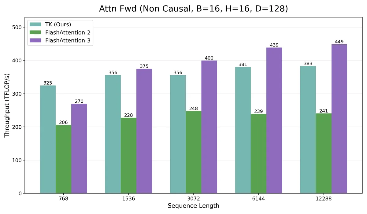
Results show very encouraging performance for such a small implementation. Our TK kernel consistently beats the PyTorch FlashAttention-2 path in this setup across all sequence lengths, by about 1.44x-1.59x, or roughly 44%-59% higher median throughput depending on sequence length. Averaged across the sweep, this comes out to around 1.55x faster.

FlashAttention-3 is still the fastest backend for the longer sequence lengths. At N=768, our TK kernel is actually ahead of FA3 in this run, but from N=1536 onward FA3 pulls ahead. Across those longer sequence lengths, TK trails FA3 by about 5%-15% of FA3 throughput, or equivalently FA3 is about 1.05x-1.17x faster.

I do want to be careful here though: this is not the same kernel that ThunderKittens reports in their paper. Their experiments use a different custom attention kernel, and they show that TK can match FlashAttention-3 performance for the same non-causal attention forward operation at some sequence lengths, and notably on the backward pass. So I would not read this benchmark as “TK versus FA3” in the absolute sense. I read it more as "with a compact implementation using the TK abstractions, we can already get very promising performance without constantly battling the lowest-level CUDA details".

Overall, I think these are very promising results, and TK is indeed a very "cute" DSL for writing AI kernels. I will definitely be experimenting with more kernels, but for now, I think this wraps up the work. I hope it was a useful read!

Massive respect and credits to everyone from Hazy Research for creating this DSL and open sourcing it. Big thanks to Benjamin Spector, Aaryan Singhal, Simran Arora, Chris Re, Stuart Sul and Nash Brown.

Please note however that this work is solely my own and I am not affiliated with Hazy Research. Please reach out if you spot any mistakes in my work; I would be happy to correct my understanding.

References

• ThunderKittens GitHub
• (Paper) ThunderKittens: Simple, Fast, and Adorable AI Kernels
• GPUs Go Brrr
• GPU Mode Lecture 77: Domain Specific Languages for GPU Kernels
• GPU Mode Lecture 75 [ScaleML Series] GPU Programming Fundamentals + ThunderKittens
• Benchmarking and Dissecting the Nvidia Hopper GPU Architecture
• NVIDIA Tensor Core Evolution: From Volta To Blackwell
• ThunderKittens: Bringing fp8 to theaters near you
• PTX Documentation
• CUTLASS Tutorial: Mastering the NVIDIA® Tensor Memory Accelerator (TMA)
• CUTLASS Tutorial: GEMM with Thread Block Clusters on NVIDIA® Blackwell GPUs
• CUTLASS Tutorial: Writing GEMM Kernels Using Tensor Memory For NVIDIA® Blackwell GPUs
• Modular Matrix Multiplication on Blackwell Series
• tcgen05 for dummies
• Outperforming cuBLAS on H100: a Worklog
• SemiAnalysis: Dissecting Nvidia Blackwell - Tensor Cores, PTX Instructions, SASS, Floorsweep, Yield
• CUTLASS Tutorial: Persistent Kernels and Stream-K
• Dynamic persistent tile scheduling with Cluster Launch Control (CLC) on NVIDIA Blackwell GPUs
• PyTorch Blog: Enabling Cluster Launch Control with TLX
• NVIDIA CUTLASS Documentation: Blackwell Cluster Launch Control
• NVIDIA CUTLASS Documentation: Work Stealing with Cluster Launch Control
• ThunderKittens Now on Blackwells!
• ThunderKittens 2.0: Even Faster Kernels for Your GPUs
• Inside NVIDIA GPUs: Anatomy of high performance matmul kernels
• FlashAttention-3