Worklog: Optimising GEMM on NVIDIA H100 for cuBLAS-like Performance (WIP)
🚧 Work in progress. Please reach out on LinkedIn if you spot any mistakes.
Introduction
Matrix multiplication sits at the core of modern deep learning. Whether it is transformers, CNNs, or even simple MLPs, everything eventually reduces to GEMM. GPUs are built to run this operation at scale, and libraries like cuBLAS set the performance bar with kernels tuned down to the last instruction.
In this blog I am rebuilding that path from the ground up on the NVIDIA H100. I start with the most basic kernels and gradually layer on optimisations: tiling into shared memory, register blocking, vectorisation, warp tiling, and then Hopper-specific features such as tensor cores, the Tensor Memory Accelerator, and more. This project is inspired by the great work of Pranjal Shankhdhar and Simon Boehm, and I try to build on from there with my own contributions, exploring the full optimisation path while providing a consistent and reproducible repository for replicating results. In the first seven kernels, we will use FP32 precision exclusively. In this phase, I wanted to focus on the fundamental optimisation techniques that form the bedrock of GEMM performance tuning and are largely architecture-independent. Using FP32 simplifies debugging with Nsight Compute and keeps PTX and SASS inspection clean. Once we enter the second phase, leveraging Tensor Cores and H100 specific features, we will transition to mixed precision. At that point, all benchmarks will compare against cuBLAS with Tensor Cores enabled, whereas in this first phase we compare against cuBLAS running in pure FP32 mode (Though they are also implemented in mixed precision in repo).
The goal is not just raw speed. It is to see what each change actually buys us, what the profiler tells us at every step, and how a kernel evolves from naive to highly tuned. By the end we will measure how close hand-rolled CUDA can get to cuBLAS, and whether on fixed matrix sizes we can even edge past it.
The full code is on my GitHub. All code is available on my GitHub with support for FP32 and BF16+FP32 mixed precision.
Let’s get started.
H100 Architecture
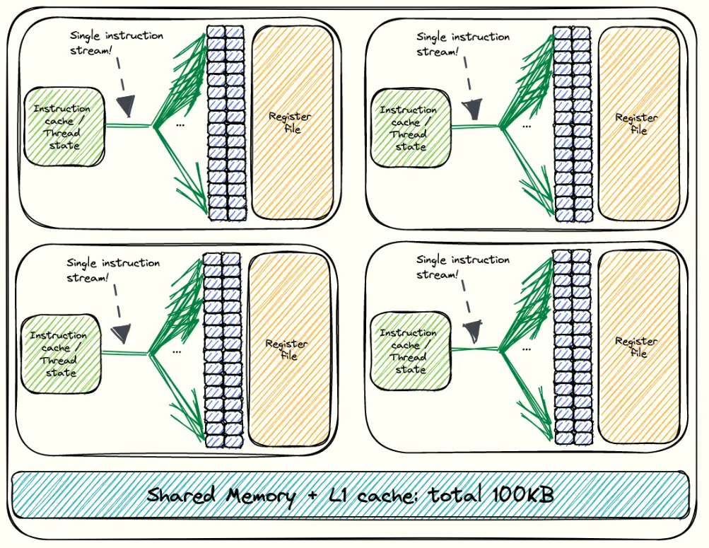
Before we get into the code, it helps to ground ourselves with a clear mental model of the GPU’s internal hardware components. Understanding the memory hierarchy within the GPU, the distinction between on-chip and off-chip memory in terms of size and latency, and the new components introduced with the Hopper architecture family will make everything that follows much easier to reason about. I won’t discuss the CUDA programming model in this section just yet; instead, I’ll introduce concepts incrementally as we move through the kernels, since I like to think of this more as a worklog. This section, then, serves more as a primer. The figure below adapted from Aleksa's post with an extension, shows the full architecture in detail.

At the top-level, the H100 is organised into multiple Graphics Processing Clusters (GPCs), we have 8 GPCs in total, and each GPC contains 18 Streaming Multiprocessors (SMs). Each four GPCs connect directly to one L2 partition and the other to second partition. These SMs hold the main compute units present on the chip along with some "on-chip" memory components. The SXM of the H100 has 132 SMs (the one I use here), while the PCIe has 114. Should actually be more than 132 SMs since 8 * 18 = 144; however, that 144 corresponds to the full GH100 die. In practice, some SMs are fused off, leaving 132 functional SMs in the SXM variant Modern GPUs such as the H100 are enormous and extremely complex pieces of silicon, making it nearly impossible to manufacture them without defects. Even a single faulty SM would make the entire chip unusable. To avoid this waste, NVIDIA fuses off defective or partially defective SMs, allowing the chip to function normally with fewer SMs. This process improves manufacturing yield. . Here is a more detailed view inside an SM:
Inside the SM, there are four partitions as shown in the illustration above. Each SM contains the following key resources:
CUDA cores: These handle the standard floating-point operations (FLOPS) and Integer operations (IOPS).
- 128 FP32 (full-precision) CUDA cores, divided logically across the four partitions (32 / partition).
- 64 INT32 cores dedicated to integer and control operations (16 / partition).
- 64 FP64 (double-precision) cores used for high-accuracy compute (16 / partition).
Fourth-generation Tensor Cores: Each SM includes 4 of these specialised units. They are designed for high-throughput matrix-multiply-accumulate operations and are essential for achieving the peak performance of modern GPU workloads.
Load/Store (LD/ST) Units: These are responsible for moving data between the SM and the memory hierarchy.
SFU Units: Handles complex math operations such as
sin,cos,sqrt, andexp, offloading this work from the CUDA cores. Each SM partition has its own SFU, enabling these operations to run in parallel with regular arithmetic. If we encounter SASS instructions that begin withMUFU(e.g.,MUFU.SQRT,MUFU.EX2), these are executed by the SFUs.Dispatch Units: These act as the bridge between the warp schedulers and the execution pipelines. Once a warp scheduler selects a warp and its next instruction, the dispatch unit routes that instruction to the appropriate functional unit within the SM. Each SM partition has its own dispatch unit, allowing multiple instructions from different warps to be issued simultaneously to different execution units.
Warp Schedulers: Each SM includes four warp schedulers (one per partition), each responsible for issuing instructions to warps — groups of 32 threads (more on that later!). A warp scheduler can issue only one instruction per clock cycle to a single warp. Across the four partitions, an SM can therefore issue up to four warp instructions per cycle, meaning 128 threads can execute in parallel at any given moment. To keep all schedulers fully utilised, we want enough active warps per block so that none sit idle. This is why we generally avoid launching fewer than 128 threads per block, as it ensures that every scheduler has a warp to work with. In practice, an SM can host multiple thread blocks and can pull warps from another block if needed, but it’s still a good heuristic to keep this in mind in cases where the SM happens to have resources for only a single block.
Now let’s look at the memory hierarchy, where each memory type physically resides within the GPU and how they differ in terms of access latency. Once again I will adapt the pyramid figure from Aleksa's post.
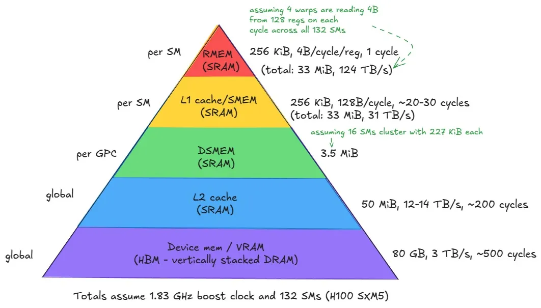
Let’s start from the bottom of the hierarchy and work our way upward, moving from the largest and slowest memories to the smallest and fastest ones.
- Global Memory (GMEM) / Device Memory (VRAM): This is the large off-chip memory sitting on the GPU package, made up of stacked HBM3 DRAM. It is generally not located on the same die as the SMs, though in modern data centre GPUs like the H100, it resides on a shared interposer alongside the GPU die to reduce latency and increase bandwidth. It uses Dynamic RAM (DRAM) cells, which are slower but denser than the Static RAM (SRAM) used in caches and registers. This memory offers the highest capacity - for instance, the H100 provides 80 GiB (≈ 687 billion bits), but also the highest latency, ≈ 500 clock cycles. Every SM accesses global memory through the L2 cache, and it serves as the backing store for all tensors/matrices. It is used to implement the GMEM of the CUDA programming model (Which we will talk about later) and to store register data that spills from the register file in the local memory.

L2 Cache: Above global memory sits the L2 cache, a large on-chip cache (made out of SRAM) shared across all SMs. It serves as the main bridge between the compute cores and the slower off-chip HBM, caching recently accessed data to reduce latency. It is physically partitioned into two parts; each SM connects directly to one partition and indirectly to the other through the crossbar.
Distributed Shared Memory (DSMEM): This is new in the memory hierarchy. DSMEM allows multiple thread blocks to share data directly across SMs within the same GPC. It extends traditional shared memory beyond a single SM, enabling cooperation between up to 16 blocks in a thread block cluster. It offers lower latency than L2 but higher than per-SM shared memory and L1 obviously.
Shared Memory (SMEM) & L1 Cache: I put these together since they co-exist on the same physical storage on-chip. They are again made out of SRAM cells, making them very fast with much lower latency and higher bandwidth than the other memory types below in the pyramid. They both have a maximum total size of 256 KiB with 31 TB/s of memory bandwidth. The L1 data cache is accessed by the LD/ST units of the SM. These 256 KiB can be configurable, by trading off a larger shared memory for a smaller L1 cache or vice versa. There is, however, a maximum of up to 228 KiB to assign for the shared memory, as we still need to have enough memory reserved for the L1 cache.Matter of fact, those 228 KiB are not exact, as seen from the H100 architecture figure above. 1 KiB of SMEM goes for system use per block anyway, so effectively, we have
228 − num_blocks * 1 KiBleft as our maximum configurable size.Register Memory (RMEM): Finally, at the lowest level of the memory hierarchy and at the top of our pyramid are the registers, which store the values manipulated by a single thread While registers are private to each thread, there is one exception: a thread can read another thread’s register, but only for threads within the same warp. This is done using warp level shuffle primitives. You can often find these in reduction kernels, for example, as they allow extremely fast communication between threads. . They are extremely fast, with effective bandwidths on the order of 124 TB/s and a latency of roughly one clock cycle. If a thread’s register usage exceeds the available register file, the compiler will spill values into local memory, which resides in global memory and is therefore much slower. As with CPU programming, registers are not directly manipulated at the CUDA C/C++ level. They are only visible in PTX and ultimately allocated by ptxas during compilation (see Compilation Story below). One of the compiler’s goals is to keep register usage per thread low enough to allow more thread blocks to reside simultaneously on an SM, since high register pressure reduces occupancy.
Tensor Memory Accelerator (TMA): Introduced with the Hopper architecture, it enables asynchronous data transfers between global memory and shared memory, as well as between shared memories within a thread block cluster. It also automatically performs swizzling to prevent shared memory bank conflicts, abstracting away the complex data movement and layout patterns that developers previously had to manage manually.
📖 Compilation Story
The journey of a CUDA program from source code to final execution is governed by a multi-stage compilation process orchestrated by the NVCC compiler driver. The NVCC compiler driver orchestrates the process, splitting the program into Host Code (CPU) and Device Code (GPU).
The Device Code is first compiled into PTX (Parallel Thread Execution) pronounced as "pee-tee-ecks" (or at least I do :)). PTX is NVIDIA's Virtual ISA (Instruction Set Architecture), which provides an architecture-independent, intermediate representation (IR) of the code. The ptxas assembler then takes the PTX code, performs necessary optimisations, and translates it into the Native ISA known as SASS (Streaming ASSembler). This is the lowest-level format in which human-readable code can be written. The SASS code, along with some other metadata are packaged into a CUBIN (CUDA Binary), which is the executable container for a specific GPU architecture. Finally, NVCC bundles one or more CUBINs together with the original PTX into a Fat Binary, which is then embedded inside the final executable alongside the CPU binary code.
The inclusion of PTX is crucial for forward compatibility: if the Fat Binary runs on a future GPU lacking a matching CUBIN, the runtime performs Just-In-Time (JIT) compilation using the embedded PTX to generate the necessary SASS, ensuring execution. We will analyse the PTX and SASS in kernels 2 and 5 to see why they are useful.

Now that we’ve built a solid mental model, let’s wrap up this section with a complete visualisation of the H100 architecture, bringing together everything we’ve discussed into perspective.

Kernel 1: Naive
In the CUDA programming model, computation is organised in a two level hierarchy. Each invocation of a CUDA kernel creates a new grid, which consists of multiple blocks. Inside each block there can be up to 1024 threads in total, regardless of whether the threads are arranged in 1D, 2D, or 3D. That is, the product blockDim.x * blockDim.y * blockDim.z <= 1024. All threads in a grid execute the same kernel function, and they rely on thread indices to distinguish themselves and to identify the appropriate portion of the data to process In general, it is recommended that the number of threads in each dimension of a thread block be a multiple of 32 for hardware efficiency reasons. They align with another concept called warps, which we will introduce soon. For now, just remember that a warp is a group of 32 threads, so keeping dimensions consistent with that is beneficial.. Kernels are written from the perspective of a single thread, following the SIMT (Single Instruction, Multiple Threads) execution model. Hence, CUDA programming is an instance of the SPMD (Single Program, Multiple Data) paradigm.
When a thread inside a kernel calls a __device__ function, it executes the function itself. It only knows about the thread that called it. Basically, it is just a normal function like in C++, but happening inside one GPU thread — and you can imagine thousands of these function instances running in parallel.
__global__ functions are the kernels. They are compiled for GPU execution but launched from the CPU (host). A kernel launch creates a grid of blocks, and each thread inside those blocks starts executing the kernel code independently.
All thread blocks operate on different parts of the input, so they can be executed in any arbitrary order. Therefore, we should never make assumptions about the execution order of blocks, or about which thread within a block will execute first.

Connecting our new understanding of the CUDA programming model with our mental model of the underlying hardware, the next diagram visualises the POV of a single thread, showing where it sits within the kernel and hardware, how it interacts with different memory spaces, and how it fits into the overall grid structure. I intentionally left out the L1 and L2 caches since they are hardware managed and not directly controlled by us.

In this first kernel, we will assign each thread in a block (within the grid) to compute exactly one element of C. Each thread takes its own coordinates and loops through the corresponding row of A across the shared dimension N (I know most official resources use K for this, but I’ve already committed to N across all kernels, so I’ll stick with that for consistency). At the same time, the thread loops down the matching column of B, accumulating the products as it goes. Once the loop is done, the result is written back into C at the same coordinates.
Spoiler alert: doing this 1-1 mapping of thread result to output is not actually the most efficient (if you guessed that, you’re right). In later kernels, we will have a single thread compute multiple elements of the output, but let’s leave this for now.
Below is a simple visualisation of how this works, including an example from the perspective of a single thread.

Notice that even though the CUDA programming model supports 2D coordinates (x, y), we still launch the block as 1D. In Simon’s work (Kernel 2), he mentions that switching from a 2D launch to a 1D launch plus remapping helps achieve coalesced global memory accesses. The idea is to launch a 1D block and then reinterpret threadIdx.x as a 2D coordinate using % and /.
However, when I tested both approaches, the 1D launch with remapping and a regular 2D launch, I observed identical performance. This initially puzzled me because Simon reported a speedup in his version. The key difference is that Simon’s naive kernel accessed matrix A down a column, which is a non-coalesced pattern, whereas his coalesced kernel accessed A across a row by letting blockIdx.x and threadIdx.x correspond to the row, not the column. This is the opposite of what I do in my version. In my implementation, even the naive kernel already accesses A in a coalesced, row-major fashion, so both versions naturally achieve the same efficiency. Funnily enough, this was probably very basic but it did confuse me for a while because I initially thought the coalescing came from the remapping trick.
So really Simon’s speedup comes from fixing the memory access pattern, not from the 1D versus 2D block layout itself. Since my naive kernel already uses coalesced loads, the launch configuration does not make a difference. I will still use the 1D launch plus remapping approach here because it gives me a natural moment to talk about memory coalescing, and I will also show how his version leads to a non-coalesced pattern. Let's just define what's a warp.
Each SM groups threads in a thread block into warps, which are sets of 32 threads. A warp is the unit of scheduling that the warp scheduler can issue instruction for only one warp at a time, and all 32 threads in that warp execute the same instruction in lockstep. Blocks are linearised into a 1D array (row-major order), then split into consecutive groups of 32 threads: warp 0 runs threads 0–31, warp 1 runs 32–63, and so on.

The code for this kernel looks like this:
template <const uint BLOCK_SIZE>
__global__ void sgemm_coalesced(const float* __restrict__ A, const float* __restrict__ B, float* __restrict__ C,
    int M, int N, int K, float alpha, float beta) {
        // flattened IDs remapping
        uint row = blockIdx.y * BLOCK_SIZE + (threadIdx.x / BLOCK_SIZE);
        uint column = blockIdx.x * BLOCK_SIZE + (threadIdx.x % BLOCK_SIZE);

        if (row < M && column < K) {
            float cumulative_sum = 0.0f;
            for (int n = 0; n < N; n++) {
                cumulative_sum += A[row * N + n] * B[n * K + column];
            }
            C[row * K + column] = (alpha * cumulative_sum) + (beta * (C[row * K + column]));
        }
    }
The remapping I mentioned happens here. If we had launched the block as two dimensional, we would simply use threadIdx.x and threadIdx.y directly, rather than computing them through threadIdx.x % BLOCK_SIZE and threadIdx.x / BLOCK_SIZE respectively.
 I like to visualise this remapping as if I was given a seat number in a cinema without being told which row or seat. Suppose each row has six seats and I am given seat number 7. Since my drawing uses 1 based numbering, I first subtract one to convert to a zero based system:
 6 = 7 - 1. Dividing by the number of seats per row gives the row index: 6 / 6 = 1, which corresponds to row 2 in 1 based indexing. The remainder tells me the seat within that row: 6 % 6 = 0, which becomes seat 1 in 1 based indexing. So seat 7 is the first seat of the second row. Dividing by the number of seats per row tells us how many complete rows we skip, and the remainder gives the seat position within that row.
uint row = blockIdx.y * BLOCK_SIZE + (threadIdx.x / BLOCK_SIZE);
uint column = blockIdx.x * BLOCK_SIZE + (threadIdx.x % BLOCK_SIZE);
Each warp of 32 threads executes the global memory load in parallel, like this:
cumulative_sum += A[row * N + n] * B[n * K + column];
Memory instructions (whether global or shared) may need to be re-issued depending on how addresses are distributed across the warp. Since we haven’t introduced shared memory yet (programming wise), let’s stay focused on global memory.
When a warp executes a load, the hardware checks if the 32 threads are accessing consecutive memory locations. The best case is when every thread reads consecutive addresses — the hardware can then coalesce all 32 requests into a single transaction.
Global memory sits in device DRAM, and DRAM is accessed in chunks of 32, 64, or 128 bytes. Fewer transactions mean higher efficiency. I’ll describe this in terms of FP32 loads (4 bytes per thread). If each thread’s 4-byte load required its own 32-byte transaction, throughput would drop by a factor of 8.
For example:
- If thread 0 reads location , thread 1 reads , thread 2 reads , … up to thread 31 reading , all 32 loads can be coalesced into a single memory transaction ().
- If the access pattern is irregular, multiple transactions may be needed, wasting bandwidth and reducing throughput.
Let us analyse the global memory access pattern for this coalesced kernel vs what a non-coalesced kernel would look like:

Running this kernel we get a throughput of 4.2 TFLOP/s, which comes out to about 8.2% relative to the FP32 cuBLAS kernel performance. We are still very far from what the hardware can theoretically deliver, often referred to as the Speed of Light (SoL)
Speed of Light refers to the theoretical upper bound on compute throughput that a GPU can deliver based purely on physics and chip design. For tensor core workloads this ceiling is given by: perf = freq_clk_max * num_tc * flop_per_tc_per_clk (989 TFLOP/s for Peak BF16 Tensor Core, 66.9 TFLOP/s for peak FP32 on H100 SXM5).
Although this number is usually presented as a fixed value, in practice it is not constant at all. It moves with the actual clock frequency the GPU can sustain, which itself changes under power and thermal limits. As a GPU approaches its power cap, the voltage regulator lowers the voltage, the clock speed drops, and the effective SoL falls with it. This behaviour is known as power throttling.
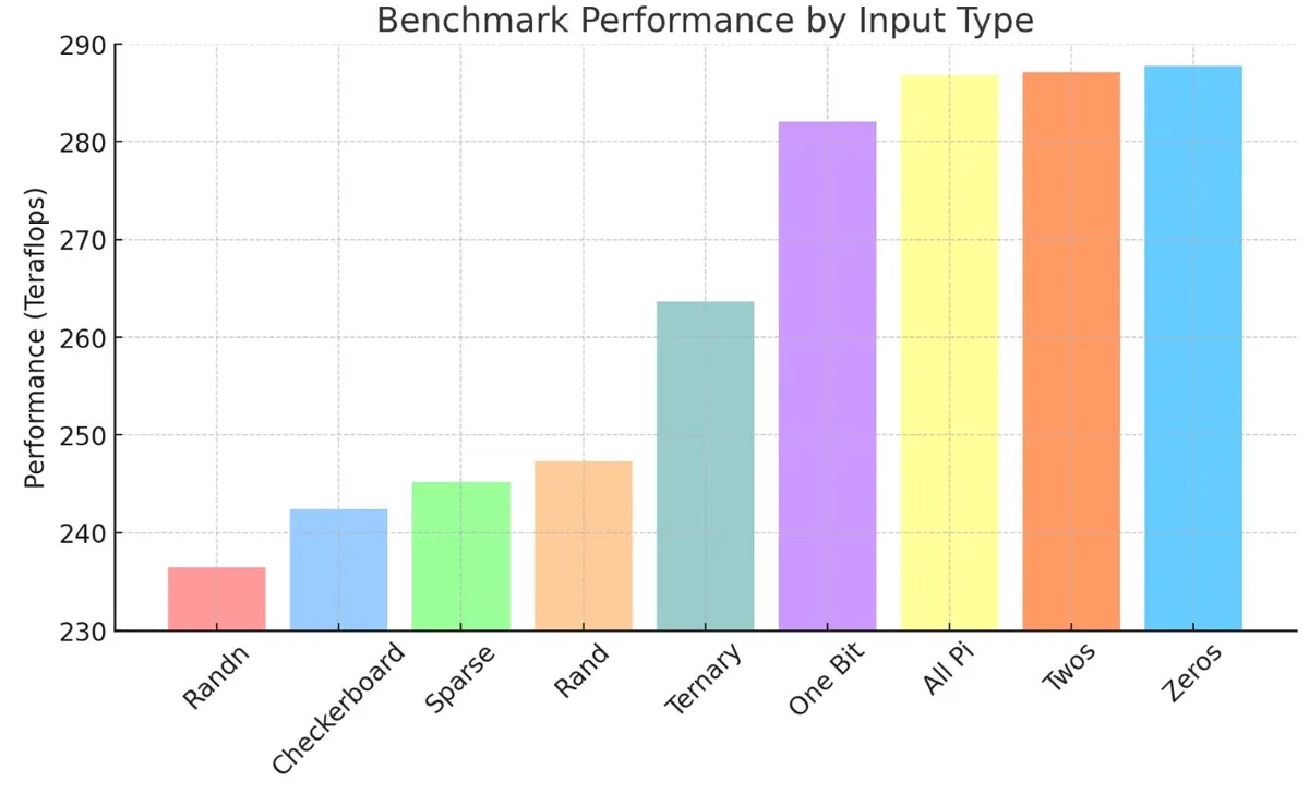
Horace He explored this beautifully using a simple matmul benchmark. A large matmul in PyTorch produced about 258 TFLOPs, while the same operation inside the CUTLASS profiler showed around 288 TFLOPs, a 10-11% improvement. It looked like a genuine kernel level speedup. But when the CUTLASS kernel was bound from Python and run with the same inputs, the gain disappeared. The only difference was that the CUTLASS profiler initialises tensors with integers, while PyTorch uses random numbers.
The reason this matters is rooted in how power is consumed on the chip. Static power keeps transistors on, while dynamic power is spent every time a transistor flips state. Random numbers cause chaotic bit flips across billions of transistors, which increases dynamic power and triggers throttling. Predictable values such as zeros or simple integer patterns flip far fewer bits, keep dynamic power low, and allow the GPU to hold higher clocks. In other words, kernels appear “faster” simply because the hardware is less electrically stressed, not because the code is more efficient.
This is why real kernels rarely reach the advertised peak TFLOP/s. The theoretical SoL assumes maximum clock frequency, but actual workloads constantly push into power and thermal constraints. The true ceiling shifts with voltage, clock speed, temperature, and even the randomness of your input data.
 . This is expected because we are still early on, and one of the most obvious bottlenecks is the fact that every iteration forces us to reach out to global memory. As mentioned earlier, accessing GMEM costs roughly 500 cycles, while accessing shared memory (SMEM) costs around 20 to 30 cycles. In the next kernel, we will improve performance by letting threads cooperatively load values from GMEM into SMEM before performing any computation. Once the tile is in SMEM, threads can fetch their operands from there instead of repeatedly going to GMEM. This speeds things up considerably and helps us move closer to higher throughput.
Kernel 2: Shared Memory Tiling
The logic behind this kernel will be as follows. We will allocate shared memory spaces for loading tiles from A and B, called sharedA and sharedB respectively. The number of elements in each tile will be TILE_SIZE * TILE_SIZE, which matches the number of threads in each block when we launch the grid with dim3 blockDim(32 * 32). This means that, just like before, each thread is responsible for computing a single element of the output. In addition to that, each thread will load two values per tile iteration, one from A and one from B, into shared memory.
I am pointing this out because later we will have kernels where each thread loads more than one element, which requires extra indexing logic to determine where that thread should write inside shared memory. In this kernel we do not need that yet, since each thread loads exactly one element from each matrix, so knowing ty and tx is enough.
This is easier to see visually than in words, so I start with a small example using 4 by 4 matrices A and B to illustrate the idea. After that I will show how the same logic looks inside the actual kernel.

Putting the logic together and applying it to our actual launch configuration, the kernel now looks like this.

The full code looks like this:
template <const uint TILE_SIZE>
__global__ void sgemm_tiled_shared(const float* __restrict__ A, const float* __restrict__ B, float* __restrict__ C,
    int M, int N, int K, float alpha, float beta) {
        // Allocate shared memory
        __shared__ float sharedA[TILE_SIZE * TILE_SIZE];
        __shared__ float sharedB[TILE_SIZE * TILE_SIZE];

        // Identify the tile of C this thread block is responsible for (We assume tiles are same size as block)
        const uint block_row = blockIdx.y;
        const uint block_column = blockIdx.x;

        // Calculate position of thread within tile (Remapping from 1-D to 2-D)
        const uint ty = threadIdx.x / TILE_SIZE; // (0, TILE_SIZE-1)
        const uint tx = threadIdx.x % TILE_SIZE; // (0, TILE_SIZE-1)

        // Move pointers from A[0], B[0] and C[0] to the starting positions of the tile
        A += block_row * TILE_SIZE * N; // Move pointer (block_row * TILE_SIZE) rows down
        B += block_column * TILE_SIZE; // Move pointer (block_column * TILE_SIZE) columns to the right
        C += (block_row * TILE_SIZE * K) + (block_column * TILE_SIZE); // Move pointer (block_row * TILE_SIZE * K) rows down then (block_column * TILE_SIZE) columns to the right

        // Calculate how many tiles we have
        const uint num_tiles = CEIL_DIV(N, TILE_SIZE);
        float cumulative_sum = 0.0f;

        // Iterate over tiles (Phase 1: Loading data)
        for (int t = 0; t < num_tiles; t++) {
            sharedA[ty * TILE_SIZE + tx] = A[ty * N + tx];
            sharedB[ty * TILE_SIZE + tx] = B[ty * K + tx];

            __syncthreads();

            // Phase 2: Compute partial results iteratively
            for (int i = 0; i < TILE_SIZE; i++) {
                cumulative_sum += sharedA[ty * TILE_SIZE + i] * sharedB[i * TILE_SIZE + tx];
            }

            __syncthreads();

            // Move all pointers to the starting positions of the next tile
            A += TILE_SIZE; // Move right
            B += TILE_SIZE * K; // Move down
        }
        // Write results back to C
        C[ty * K + tx] = (alpha * cumulative_sum) + (beta * C[ty * K + tx]);
    }
While this kernel achieves approximately a 1.7× throughput improvement over the previous kernel and now reaches 13.9% relative to cuBLAS (FP32), profiling it with Nvidia’s Nsight Compute reveals a few key problems.
First, if we look at the Speed of Light section in the profiler we notice something interesting. We get 76.63% Compute throughput and a Memory throughput of 91.13%. These are percentages relative to the SoL of the hardware on FP32. This sounds confusing, as at first 76.63% compute throughput may seem very decent, but this is a relatively basic GEMM kernel so it cannot make sense.
Looking at the throughput breakdown, which shows the bottlenecks in percentage terms, we instantly understand the misconception. SM: Inst Executed Pipe Lsu = 76.63% (the same number as shown in the overview because the overview simply displays the highest percentage across the instruction breakdown). Pipe LSU is the load store unit. As the profiler describes, its role is
"The LSU pipeline issues load, store, atomic, and reduction instructions to the L1TEX unit for global, local, and shared memory. It also issues special register reads (S2R), shuffles, and CTA level arrive or wait barrier instructions to the L1TEX unit."
The next highest issued instructions are SM: Mio Inst Issued at 40.08% which is the memory input or output unit. This means instruction issue is split almost half between LSU operations and non memory operations, again pointing to the memory side being the dominant force.
What about the number of instructions doing FP32 computation? SM: Pipe FMA Cycles Active = 14.81%. This is the real number we care about because it shows we are nowhere near utilising our FP32 hardware capability at all, which is exactly what we should expect this early on. This metric answers the question of on what fraction of active SM cycles the FP32 FMA execution pipe was actually doing work. For a good GEMM, we would love to see this number very high (think 60 to 80%+) because GEMM is almost all FMAs. Spoiler alert: we will see in kernel six how we increase this number to 62%.
The overview compute throughput number (the one selected as the maximum) was therefore a bit misleading because the overall value considers all instructions executed on the SM (ALU, FMA, SFU, LSU and so on). There are other useful metrics as well, but we will ignore them for now. I have all the profiling reports in downloadable .ncu-rep format in the GitHub repository if you want to open them in Nsight Compute and inspect them in detail. For now let us turn our attention to the memory throughput breakdown.
Our top three metrics are L1: Data Pipe Lsu Wavefronts = 91.13%, L1: Lsu Writeback Active = 87.07% and L1: Lsuin Requests = 76.63%. At this point it is obvious we are simply overwhelming shared memory with the sheer amount of loads and stores we request to and from it.
There are still interesting metrics and angles to look at this from the profiler so the below figure will show three different views from the profiler annotated. For the SASS code, you can view the full SASS code of this kernel either from the profiler itself in the source section or from this GoodBolt link.

As I point out in the roofline plot
 Arithmetic intensity is the ratio of arithmetic operations to memory operations in a kernel.
, we want to increase arithmetic intensity, or visually move to the right on the plot. Due to the high ratio between arithmetic bandwidth and memory bandwidth in modern GPUs, the most efficient kernels have high arithmetic intensity. This means that when we address a memory bottleneck, we can often shift work from the memory subsystem to the compute subsystem, saving on memory bandwidth while increasing the load on the arithmetic units.
Arithmetic intensity is the ratio of arithmetic operations to memory operations in a kernel.
, we want to increase arithmetic intensity, or visually move to the right on the plot. Due to the high ratio between arithmetic bandwidth and memory bandwidth in modern GPUs, the most efficient kernels have high arithmetic intensity. This means that when we address a memory bottleneck, we can often shift work from the memory subsystem to the compute subsystem, saving on memory bandwidth while increasing the load on the arithmetic units.
Therefore, in our next kernel, instead of letting each thread compute the result of just one element in the output matrix, we will let it compute multiple elements. Each thread will partially accumulate several results in its own registers and only once the computation is complete will it store the final values back from registers into C.
Kernel 3: 1D Register Tiling
Write up in progress. All code for kernels are available on GitHub.

Kernel 4: 2D Register Tiling
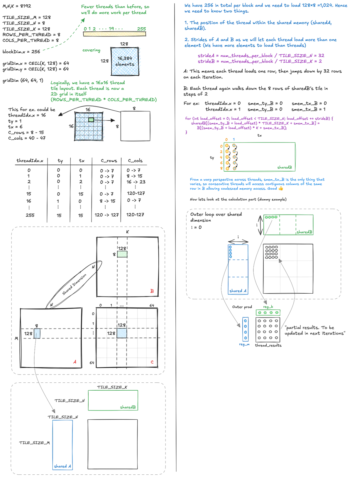
To squeeze in a little more arithmetic intensity in our kernel we now let each thread compute more than a single output element. As illustrated below, the idea is that a thread block covers a tile of the output matrix and inside that tile each thread is responsible for its own small 2D patch, computing ROWS_PER_THREAD * COLS_PER_THREAD results.
Since we now launch fewer threads than the number of elements in the shared memory tiles, each thread must load multiple elements from global memory into shared memory, using a stride so that all elements of the tiles are covered without overlap. Once the shared memory tiles for A and B are fully populated, each thread repeatedly loads the pieces of A and B it needs from shared memory into registers, performs partial outer product updates, and accumulates into its local registers until its final ROWS_PER_THREAD * COLS_PER_THREAD block of C is complete.
The code for this kernel looks like this:
template <const uint TILE_SIZE_M, const uint TILE_SIZE_N, const uint TILE_SIZE_K, const uint ROWS_PER_THREAD>
__global__ void sgemm_1D_registertiling(const float* __restrict__ A, const float* __restrict__ B, float* __restrict__ C,
    int M, int N, int K, float alpha, float beta) {

    // Allocate shared memory
    __shared__ float sharedA[TILE_SIZE_M * TILE_SIZE_N];
    __shared__ float sharedB[TILE_SIZE_N * TILE_SIZE_K];

    // Identify the tile of C this thread block is responsible for
    const uint block_row = blockIdx.y;
    const uint block_column = blockIdx.x;

    // Calculate position of thread within tile (Remapping from 1-D to 2-D)
    const uint ty = threadIdx.x / TILE_SIZE_K;
    const uint tx = threadIdx.x % TILE_SIZE_K;

    // Move pointers from A[0], B[0] and C[0] to the starting positions of the tile
    A += block_row * TILE_SIZE_M * N;
    B += block_column * TILE_SIZE_K;
    C += (block_row * TILE_SIZE_M * K) + (block_column * TILE_SIZE_K);

    // Calculate position of thread within shared memory tile
    const uint smem_ty_A = threadIdx.x / TILE_SIZE_N;
    const uint smem_tx_A = threadIdx.x % TILE_SIZE_N;

    const uint smem_ty_B = threadIdx.x / TILE_SIZE_K;
    const uint smem_tx_B = threadIdx.x % TILE_SIZE_K;

    // Calculate number of tiles
    const uint num_tiles = CEIL_DIV(N, TILE_SIZE_N);

    // Initialise thread-local results in registers
    float thread_results[ROWS_PER_THREAD] = {0.0f};

    // Iterate over tiles
    for (int t = 0; t < num_tiles; t++) {
        sharedA[smem_ty_A * TILE_SIZE_N + smem_tx_A] =
            A[smem_ty_A * N + smem_tx_A];

        sharedB[smem_ty_B * TILE_SIZE_K + smem_tx_B] =
            B[smem_ty_B * K + smem_tx_B];

        __syncthreads();

        // Inner computation loop
        for (int i = 0; i < TILE_SIZE_N; i++) {
            float fixed_B = sharedB[i * TILE_SIZE_K + tx];
            for (int row = 0; row < ROWS_PER_THREAD; row++) {
                uint global_row_idx = ty * ROWS_PER_THREAD + row;
                thread_results[row] +=
                    sharedA[global_row_idx * TILE_SIZE_N + i] *
                    fixed_B;
            }
        }

        __syncthreads();

        // Move to next tile
        A += TILE_SIZE_N;
        B += TILE_SIZE_N * K;
    }

    // Write results back to C
    for (int row = 0; row < ROWS_PER_THREAD; row++) {
        uint global_row_idx = ty * ROWS_PER_THREAD + row;
        C[global_row_idx * K + tx] =
            (alpha * thread_results[row]) +
            (beta * C[global_row_idx * K + tx]);
    }
}
Last kernel reduced memory IO stalls, but we were still doing too many shared memory reads per thread per output:
- 9108 SMEM reads per output
- 254 GMEM reads per output
In this kernel, each thread now computes a tile of rows and columns, not just a vertical strip. That brought it down to:
- 2024 SMEM reads per output
- 128 GMEM reads per output
That is a 4.5x reduction in SMEM load traffic per output and 2× in GMEM, while computing 8× more results per thread.
Profiling this kernel shows that it reaches 38% of the H100’s FP32 peak, which immediately tells us we are not compute-bound. Global memory is also nowhere near saturated: the kernel uses only 2.90% of DRAM bandwidth and about 10.13% of L2, both extremely low for a GEMM workload. So neither global bandwidth nor L2 traffic is limiting anything.
The first meaningful signal appears in the Speed of Light section:
- Compute Throughput: 55.50%
- Memory Throughput: 85.88%
- L1/TEX Throughput: 87.74%
The profiler even points us directly toward the bottleneck:
“The kernel is utilising greater than 80% of the available compute or memory performance. To further improve performance, work will likely need to be shifted from the most utilised unit to another. Start by analysing L1 in the Memory Workload Analysis section.”
Since DRAM and L2 are barely touched while L1/TEX is approaching 90% utilisation, the pressure is clearly concentrated in the on-chip memory hierarchy. In other words, this is not DRAM problem at all. The limiting factor is the bandwidth and latency of the L1 cache/SMEM path.
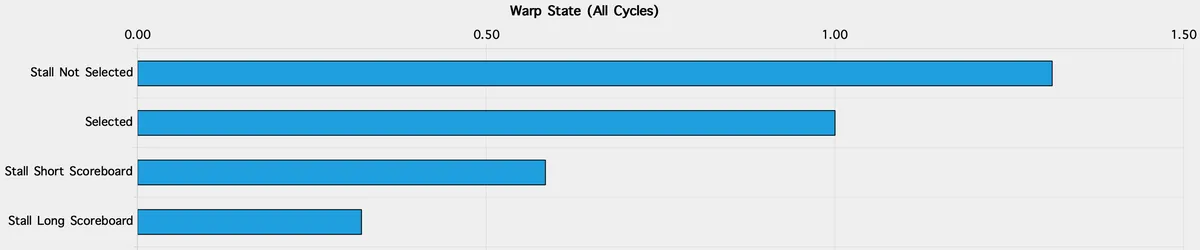
This picture is reinforced by the scheduler metrics. SM Issue Active is 55.50%, meaning the warp scheduler issues instructions for just over half of all cycles. The remaining ~45% of cycles are spent stalled, typically waiting on data movement through L1/SMEM rather than through DRAM or L2.
Looking at the scheduler statistics we find:
"Every scheduler is capable of issuing one instruction per cycle, but for this kernel each scheduler only issues an instruction every 1.8 cycles. This might leave hardware resources underutilized and may lead to less optimal performance."
The Stall MIO throttle is also on 0.59, so we want to reduce this. Taken together: extremely low DRAM usage, extremely low L2 usage, high L1/TEX utilisation (∼88%), and only mid-50% SM issue all converge to the same conclusion. In this
This kernel is L1-bound or SMEM-bound. It is not compute-bound, and it is certainly not GMEM-bound. The bottleneck is the on-chip data movement between registers, shared memory, and the L1/TEX path. Our next optimisation will require reducing the instruction overhead within the L1/SMEM pipeline, directly addressing the 1.8 cycles per instruction rate and freeing the warp scheduler to increase SM Issue Active.
Despite the limitations, we still land a 1.40× gain over the previous kernel: 19.1 TFLOPs versus 12.2 TFLOPs, pushing us up to 36.8% of cuBLAS.
Kernel 5: Vectorised 2D Register Tiling
Up until now, in all our previous kernels we issued one load instruction per scalar. It is slightly confusing because the coalescing we optimised for might suggest that we are not really doing one load per scalar. The missing detail is that there is an important distinction between:
- memory transactions
- the number of instructions issued
Coalescing only helps with the first point. It allows the hardware to merge the data requested by different threads into a single contiguous memory transaction. It does not change the second point at all. Every scalar load still appears as a separate instruction, and each one must be issued by the warp scheduler and pushed through the load and store pipeline.
To confirm this, inspecting the SASS of the previous kernel, specifically the parts where we load from GMEM to SMEM, we do in fact find that every loop iteration generates a separate instruction issue per thread. While we know the accesses to B for example are coalesced, which achieves its purpose at the memory controller level, the hardware still requires four separate instruction issues per threadCoalescing does not happen at compile time. The hardware performs it dynamically at runtime once the actual addresses are known. This is sensible, since the compiler cannot assume alignment or layout since our matrix pointers are passed in as function arguments.. Now, extrapolate this across the whole warp: every time the kernel cycles through this section, the warp scheduler must issue a total of 32 threads * 4 loads/thread = 128 separate load instructions. Even though the memory controller may merge all those 128 scalar requests into a handful of large, efficient memory transactions, the pipeline bottleneck remains at the frontend. The warp scheduler is overworked, and the load/store pipeline is saturated with repetitive requests, starving the actual compute units of valuable clock cycles.

The only way to resolve the instruction pressure is to fundamentally change how the compiler views the data transfer. We must tell the compiler that when it sees a single load request, it should fetch multiple scalars at once. CUDA offers vectorised variables that allow us to reduce this instruction pressure. These refer to wider data types such as float2 or float4. A regular float is 32 bits (4 bytes). A float4 is 128 bits (16 bytes). By casting a float* to a float4* and issuing a single load, we trigger one 128-bit global memory instruction. In SASS this appears as LDG.E.128 and sometimes LDG.E.CI.128. This reduces the load instruction count dramatically and makes more efficient use of the hardware memory paths.
Let’s look at the next kernel then. The whole structure remains the same, the only difference is that we will transpose sharedA. So loading a row from GMEM will be stored in sharedA as a column. We do this to allow us to use vectorised loads, since issuing a vectorised load instruction requires the addresses to be physically contiguous.
The logic centres on the access pattern for Matrix A. Since each thread needs to load the ROWS_PER_THREAD elements required for its calculation (which correspond to traversing a column), the default memory accesses are strided. If we transpose the column data, it will be physically stored as a contiguous row in sharedA. This allows us to issue float4 loads later when moving data from the SMEM to reg_m.
The same approach applies for sharedB, but we won't be transposing it. As we recall from the last kernel, each thread loads COLS_PER_THREAD into reg_k, and these elements are already next to each other on the same row, so we don't need to transpose.
What doing this leads to is the complete abandonment of the scalar + offset approach, and so we won't need to loop with strides to load from GMEM to SMEM. This also means that when we load into registers, since we can issue float4 and both ROWS_PER_THREAD and COLS_PER_THREAD are 8, we will still load into registers in a loop but will now stride in steps of 4. This all might sound confusing, so as usual, I will draw it visually.


Now let’s inspect the SASS for this kernel, compare it with the previous version, and then look at what the profiler tells us.

We can see that the number instructions issued per thread dropped from 8 to just 2 using our approach. The visual above shows only the GMEM loading phase with LDG.E.CI.128, but similarly we cut down the number of instructions when reading from SMEM to RMEM (Register Memory). While I won't put it here because it's much longer, we can clearly still see the LDS.U.128 instruction in the SASS, confirming the success of vectorising the shared memory reads as well. You can still see the full SASS/PTX for this kernel if you are interested to look into it more.
Running this kernel we get another ≈2x speedup and now at 72% of cuBLAS performance with 37.2 TFLOP/s. Great, we are getting there (FP32 path only ofc yet! still a long way to beat cuBLAS with tensor cores)
The profiler shows the kernel is now making reasonably good use of our GPU, compute throughput sits around 66% of peak, memory throughput around 85%, and we’re hitting 56% of the device FP32 roofline.
Bare in mind cuBLAS sits at around 85%, and no practical workload would actually reach 100% of the hardware theoretical peak.
Now let's compare the issues we found before with our new profiler results for this kernel:
SM Issue Active: Increased from 55.50% to 66.05% (More time spent on compute. The scheduler is ∼19% busier).SM Pipe Fma Cycles Active: Increased from 42.00% to 56.73% (More computations are being done).SM Inst Executed Pipe Lsu(Load Store Unit): Decreased from 28.78% to 17.09% (Evidence of the instruction count drop).SM Mio Inst Issued: Decreased from 14.99% to 9.21%.Stall MIO Throttle: Decreased from 0.59 to 0.02.
Furthermore, the warning regarding the scheduler issuing only 1.8 cycles per instruction is now gone. Massive improvements, but there are still improvements to be made.
Looking carefully, there are some key metrics subtleties that are hurting our current performance and holding us back from achieving higher compute throughput.
Most critically, shared memory accesses show heavy bank conflicts: about 5-way conflicts on loads and 2.6-way conflicts on stores, with over 40% of all shared memory wavefronts wasted in serialisation.
In Nsight Compute, a wavefront refers to the hardware chunk of shared memory requests that can be handled in a single cycle. When bank conflicts occur, the request must split into multiple wavefronts, each processed one after the other, causing stalls.
We haven’t really considered bank conflicts yet in our kernels, so this is a suitable time to introduce the concept.

I tried to draw the shared memory organisation to visualise this better, but the key concept to grasp is that shared memory on NVIDIA GPUs (including H100) is divided into 32 banks, each of which can serve one 4-byte word per cycle. I like to think of it like thirty-two checkout lanes at a supermarket, with each lane handling one customer per cycle. A “word” here just means the basic unit of storage: 4 bytes (so a single float for ex).
The bank index can then be simply calculated using the common modulo trick:
bank_index = word_index % 32
- Bank 0: words 0, 32, 64, …
- Bank 1: words 1, 33, 65, …
- …
- Bank 31: words 31, 63, 95, …
Now, when a warp of 32 threads issues a shared memory access:
- If each thread touches a different bank, no conflict, everyone gets served in parallel. Good!
- If multiple threads try to read/write different addresses in the same bank, those requests are serialised, one after another. That’s a bank conflict.
- If all threads read the exact same word, the hardware does a broadcast instead, which is efficient. Also good!
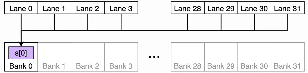 In this diagram, all 32 lanes can read from the same banked word.
The hardware broadcasts the value efficiently instead of causing a conflict.
In this diagram, all 32 lanes can read from the same banked word.
The hardware broadcasts the value efficiently instead of causing a conflict.

Let us start with the store conflicts. In our code the ≈ 2.6 conflicts on stores show up when we populate sharedA with the transposed tile.
// Populate smem using vector loads
float4 tempA = reinterpret_cast<const float4*>(&A[smem_ty_A * N + smem_tx_A*4])[0]; // [0] dereference issues one ld.global.nc.v4.f32

// Transpose A (instead of 128x8 previously for ex, now it will be 8x128)
sharedA[(smem_tx_A * 4 + 0) * TILE_SIZE_M + smem_ty_A] = tempA.x;
sharedA[(smem_tx_A * 4 + 1) * TILE_SIZE_M + smem_ty_A] = tempA.y;
sharedA[(smem_tx_A * 4 + 2) * TILE_SIZE_M + smem_ty_A] = tempA.z;
sharedA[(smem_tx_A * 4 + 3) * TILE_SIZE_M + smem_ty_A] = tempA.w;
smem_ty_A ranges across the columns in our transposed sharedA and smem_tx_A is either 0 or 1 (in this kernel configuration ofc). The word index for each scalar store is:
word_index = (smem_tx_A*4 + q) * TILE_SIZE_M + smem_ty_A→ q in {0,1,2,3}bank = word_index % 32
With TILE_SIZE_M = 128, the leading stride is divisible by 32 banks. Because 128 % 32 = 0, the bank depends only on the offset that survives the calculation, not on the stride factor.
The bank effectively depends only on the smem_ty_A value (the column offset) and not on the smem_tx_A value (the row index). Since each two threads share the same smem_ty_A value, they all target the same bank for each of the four scalar stores. This is exactly the pattern the profiler called out as two-way store conflicts.
One common trick to avoid this class of conflict when the leading stride is a multiple of 32 words is padding.
// Allocate shared memory. Use padded leading strides that keep float4 alignment
constexpr uint STRIDE_A = (TILE_SIZE_M % 32u == 0u) ? (TILE_SIZE_M + 4u) : TILE_SIZE_M;
constexpr uint STRIDE_B = (TILE_SIZE_K % 32u == 0u) ? (TILE_SIZE_K + 4u) : TILE_SIZE_K;
static_assert((STRIDE_A % 4u) == 0u, "STRIDE_A must keep float4 alignment");
static_assert((STRIDE_B % 4u) == 0u, "STRIDE_B must keep float4 alignment");
If we pad the leading stride to 132 words and use that padded stride everywhere we touch sharedA (both when writing the transpose and when reading it later), the index driving the row smem_tx_A now influences the bank. The two lanes that used to collide are split onto sixteen banks apart, and the four scalar stores for x, y, z, w rotate across banks rather than piling onto one. To prove this, I profiled the kernel after padding and the results showed store conflicts were eliminated.

Now we still have the actually bigger conflict which is the five-way bank conflict for the loads. The conflict mainly happens when loading from sharedB, particularly at:
for (int col = 0; col < COLS_PER_THREAD; col += 4) {
  uint global_smem_col_idx = tx * COLS_PER_THREAD + col;
  float4 temp_shared_B =
      reinterpret_cast<float4*>(&sharedB[i * TILE_SIZE_K + global_smem_col_idx])[0];
  reg_k[col + 0] = temp_shared_B.x;
  reg_k[col + 1] = temp_shared_B.y;
  reg_k[col + 2] = temp_shared_B.z;
  reg_k[col + 3] = temp_shared_B.w;
}
For lanes 0..15, ty is still 0 but tx walks 0..15. If we freeze col = 0 to make it simple, the bank for the first word of each lane’s float4 will be:
bank = (i* 128 + 8 * tx) % 32 = (8 * tx) % 32- = 0, 8, 16, 24, 0, 8, 16, 24, ... only four banks used by a half warp
Now remember we are doing vectorised float4 loads so it spans four consecutive banks for that lane. So lane with bank start 0 touches banks {0,1,2,3}, lane with 8 touches {8,9,10,11}, lane with 16 touches {16,17,18,19}, lane with 24 touches {24,25,26,27}, and so on.
Since the pattern repeats every four lanes, that means we have four lanes that all want banks {0..3} at the same time, four lanes that all want {8..11}, etc. This is where we get a four-way conflict for this instruction.
For sharedA loads it’s different. What varies across lanes inside a half warp is tx, but tx does not appear in the address. Inside one half warp ty is constant. For fixed i and row, every lane computes the same address. So all sixteen lanes in the half warp read the same four words of sharedA at that step. As I said earlier this can be broadcasted, so it’s conflict-free in terms of load.

The important bit here is that padding does not fix this load conflict. Padding helps when the varying part of the address is multiplied by a stride that is a multiple of thirty-two words. In the sharedB load above, the varying part is tx * COLS_PER_THREAD + col, and that bit is not multiplied by the padded stride. So even if we set STRIDE_B = 132, the lanes inside a half warp still bunch onto the same four bank groups. So, padding solved the store side, but the sharedB load conflicts need a different approach.
The final code for our padded vectorised 2D register tiling kernel looks like this:
template <const uint TILE_SIZE_M, const uint TILE_SIZE_N, const uint TILE_SIZE_K, const uint ROWS_PER_THREAD, const uint COLS_PER_THREAD>
__global__ void sgemm_vectorised(const float *__restrict__ A, const float *__restrict__ B, float *__restrict__ C,
                                 int M, int N, int K, float alpha, float beta)
{
    // Allocate shared memory. Use padded leading strides that keep float4 alignment
    constexpr uint STRIDE_A = (TILE_SIZE_M % 32u == 0u) ? (TILE_SIZE_M + 4u) : TILE_SIZE_M;
    constexpr uint STRIDE_B = (TILE_SIZE_K % 32u == 0u) ? (TILE_SIZE_K + 4u) : TILE_SIZE_K;
    static_assert((STRIDE_A % 4u) == 0u, "STRIDE_A must keep float4 alignment");
    static_assert((STRIDE_B % 4u) == 0u, "STRIDE_B must keep float4 alignment");

    // Allocate shared memory
    __shared__ float sharedA[STRIDE_A * TILE_SIZE_N];
    __shared__ float sharedB[TILE_SIZE_N * STRIDE_B];

    // Identify the tile of C this thread block is responsible for
    const uint block_row = blockIdx.y;
    const uint block_column = blockIdx.x;

    // Calculate position of thread within tile (Remapping from 1-D to 2-D)
    const uint ty = threadIdx.x / (TILE_SIZE_K / COLS_PER_THREAD);
    const uint tx = threadIdx.x % (TILE_SIZE_K / COLS_PER_THREAD);

    // Move pointers from A, B, C to tile starts
    A += block_row * TILE_SIZE_M * N;
    B += block_column * TILE_SIZE_K;
    C += (block_row * TILE_SIZE_M * K) + (block_column * TILE_SIZE_K);

    // Map each thread to one 4-float chunk
    const uint smem_ty_A = threadIdx.x / (TILE_SIZE_N / 4);
    const uint smem_tx_A = threadIdx.x % (TILE_SIZE_N / 4);

    const uint smem_ty_B = threadIdx.x / (TILE_SIZE_K / 4);
    const uint smem_tx_B = threadIdx.x % (TILE_SIZE_K / 4);

    // Tile count
    const uint num_tiles = CEIL_DIV(N, TILE_SIZE_N);
    float thread_results[ROWS_PER_THREAD * COLS_PER_THREAD] = {0.0f};
    float reg_m[ROWS_PER_THREAD] = {0.0f};
    float reg_k[COLS_PER_THREAD] = {0.0f};

    // Outer loop iterate over tiles
    for (int t = 0; t < num_tiles; t++)
    {
        // Populate smem using vector loads
        float4 tempA = reinterpret_cast<const float4 *>(&A[smem_ty_A * N + smem_tx_A * 4])[0];
        sharedA[(smem_tx_A * 4 + 0) * STRIDE_A + smem_ty_A] = tempA.x;
        sharedA[(smem_tx_A * 4 + 1) * STRIDE_A + smem_ty_A] = tempA.y;
        sharedA[(smem_tx_A * 4 + 2) * STRIDE_A + smem_ty_A] = tempA.z;
        sharedA[(smem_tx_A * 4 + 3) * STRIDE_A + smem_ty_A] = tempA.w;

        float4 tempB = reinterpret_cast<const float4 *>(&B[smem_ty_B * K + smem_tx_B * 4])[0];
        reinterpret_cast<float4 *>(&sharedB[smem_ty_B * STRIDE_B + smem_tx_B * 4])[0] = tempB;

        __syncthreads();

        // Outer loop over shared dimension N
        for (int i = 0; i < TILE_SIZE_N; i++)
        {
            // Load regs from sharedA
            for (int row = 0; row < ROWS_PER_THREAD; row += 4)
            {
                uint global_smem_row_idx = ty * ROWS_PER_THREAD + row;
                float4 temp_shared_A = reinterpret_cast<float4 *>(&sharedA[i * STRIDE_A + global_smem_row_idx])[0];
                reg_m[row + 0] = temp_shared_A.x;
                reg_m[row + 1] = temp_shared_A.y;
                reg_m[row + 2] = temp_shared_A.z;
                reg_m[row + 3] = temp_shared_A.w;
            }

            // Load regs from sharedB
            for (int col = 0; col < COLS_PER_THREAD; col += 4)
            {
                uint global_smem_col_idx = tx * COLS_PER_THREAD + col;
                float4 temp_shared_B = reinterpret_cast<float4 *>(&sharedB[i * STRIDE_B + global_smem_col_idx])[0];
                reg_k[col + 0] = temp_shared_B.x;
                reg_k[col + 1] = temp_shared_B.y;
                reg_k[col + 2] = temp_shared_B.z;
                reg_k[col + 3] = temp_shared_B.w;
            }

            // Outer product
            for (uint m = 0; m < ROWS_PER_THREAD; m++)
                for (uint k = 0; k < COLS_PER_THREAD; k++)
                    thread_results[m * COLS_PER_THREAD + k] += reg_m[m] * reg_k[k];
        }

        __syncthreads();

        A += TILE_SIZE_N;
        B += TILE_SIZE_N * K;
    }

    // Write results back
    for (uint row = 0; row < ROWS_PER_THREAD; row++)
        for (uint col = 0; col < COLS_PER_THREAD; col += 4)
        {
            uint global_row_idx = ty * ROWS_PER_THREAD + row;
            uint global_col_idx = tx * COLS_PER_THREAD + col;
            float4 tempC = reinterpret_cast<float4 *>(&C[global_row_idx * K + global_col_idx])[0];

            tempC.x = (alpha * thread_results[row * COLS_PER_THREAD + col]) + (beta * tempC.x);
            tempC.y = (alpha * thread_results[row * COLS_PER_THREAD + col + 1]) + (beta * tempC.y);
            tempC.z = (alpha * thread_results[row * COLS_PER_THREAD + col + 2]) + (beta * tempC.z);
            tempC.w = (alpha * thread_results[row * COLS_PER_THREAD + col + 3]) + (beta * tempC.w);

            reinterpret_cast<float4 *>(&C[global_row_idx * K + global_col_idx])[0] = tempC;
        }
}
Kernel 6: Warp Tiling
So far we exploited two levels of parallelism.
- Block tiling: Each thread block computed a large tile of the output matrix C, reusing tiles of A and B from shared memory.
- Register tiling: Each thread computed a small sub-tile of C
(ROWS_PER_THREAD × COLS_PER_THREAD)entirely in registers, maximising data reuse before writing results back to global memory.
For this kernel, we will introduce a new level of tiling between block tiling and thread tiling and that is warp tiling.
Warp tiling sits between block tiling and thread tiling in the optimisation hierarchy. Instead of having all threads in a block cooperatively work on one large tile, we partition that tile into smaller sub-tiles, each assigned to a warp. This turns the warp into the middle-level unit of computation. The block still covers a 128 × 128 patch of C, but we split it into four 64 × 64 sub-tiles. Two warps along M by two warps along K which give us four warps per block.
TILE_SIZE_M = 128
TILE_SIZE_N = 16
TILE_SIZE_K = 128

WARP_TILE_M  = 64
WARP_TILE_K  = 64
WARP_STEPS_K = 4

ROWS_PER_THREAD = 8
COLS_PER_THREAD = 4
NUM_THREADS     = 128   // four warps per block
The block still works cooperatively to load data from GMEM into SMEM (using the vectorised, padded, and transposed techniques from the previous kernel). Once the data is on-chip, the threads split into four warps, with each warp taking exclusive ownership of one quadrant of the output matrix, identified by warp_row and warp_col.
The 32 threads within a warp utilise their specific sub-indices (ty, tx derived from the 8×4 thread sub-grid) to attack their assigned 64×64 region. The warp covers the vertical dimension in one pass WARP_STEPS_M = 1 but must iterate horizontally WARP_STEPS_K=4 times (These are configurable ofc but need to be done carefully!). The partial results accumulation occurs within the loop that iterates over the TILE_SIZE_N shared dimension (i loop). In the compute loop, this design allows the thread to load the reg_m fragment from sharedA once and reuse it across the four horizontal steps, loading fresh reg_k data from sharedB for each step before summing the results of the outer product (between reg_m and reg_k) into the large thread_results array, accumulating the final result across all i iterations.
I will start by showing the high-level structure of the kernel, illustrating how warp tiling integrates as our new level of hierarchy. Following that, we will take the POV of a single thread using some dummy parameters, to visualise this thread's entire lifetime: where its computation happens, and exactly where it performs its loads and stores.

Now, we visualise the flow of computation from a single thread's perspective.

This extra level of tiling provides several benefits:
Alignment with hardware scheduling:
The warp is the fundamental execution unit in NVIDIA GPUs. By giving each warp its own sub-tile of the output, we align our work partitioning with the way the hardware actually schedules instructions.
By doing so, each warp can execute independently. If one warp stalls on memory, others can continue executing, which keeps warp scheduler slots full and reduces idle cycles.
 From Simon's blog
Control over shared memory access
Warp tiles keep each warp’s footprint compact and the per-lane strides simple and repeatable. That makes it easier to design bank-friendly layouts. Spoiler alert! that’s why SMEM load conflicts didn’t show up for this kernel.
Improved register cache locality
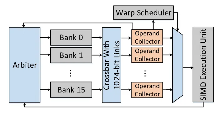
The register file (RF) inside each Streaming Multiprocessor stores per-thread variables. On Hopper, it’s split into multiple single-ported banks (similar to SMEM banks!). A bank can only serve one access per cycle. If two threads in the same warp try to read from the same bank in the same cycle, the accesses are serialized. This is called a bank conflict as well but for registers and it increases the time it takes to fetch operands for an instruction. Unfortunately NVIDIA’s profiling tools don’t provide metrics for these conflicts so it is hard to verify whether that was something we actually improved in this kernel.
Between the RF and the execution units are Operand Collector Units (OCUs) Paper: BOW Breathing Operand Windows to Exploit Bypassing in GPUs . Each OCU fetches source operands from the register banks and stores them in a small buffer, with space for three 128-byte entries. If an operand is needed again soon, it can be served directly from this buffer instead of going back to the main RF. This avoids both bank conflicts and extra RF traffic.
Warp tiling helps here because each warp works on a small, fixed sub-tile of the output matrix, so it tends to reuse the same registers repeatedly in the inner loop. This makes bank conflicts less likely and increases the chances that operands can be reused directly from the OCU buffer.
Again this is a speculation, Idk really if it makes a difference, but it seems plausible.
The main parts of the code that changed looks like this:
// Iterate over the shared dimension of the SMEM tiles
for (int i = 0; i < TILE_SIZE_N; i++)
{
// Load slice at current i iteration in sharedA's register
for (int wSubRow = 0; wSubRow < WARP_STEPS_M; wSubRow++)
{
uint base_row =
(warp_row * WARP_TILE_M) +
(wSubRow * WARP_SUB_M) +
(ty * ROWS_PER_THREAD);
// Each thread loads ROWS_PER_THREAD into the register
for (int row = 0; row < ROWS_PER_THREAD; row += 4)
{
const float4 va =
reinterpret_cast<const float4*>(
&sharedA[i * STRIDE_A + base_row + row])[0];
reg_m[wSubRow * ROWS_PER_THREAD + row + 0] = va.x;
reg_m[wSubRow * ROWS_PER_THREAD + row + 1] = va.y;
reg_m[wSubRow * ROWS_PER_THREAD + row + 2] = va.z;
reg_m[wSubRow * ROWS_PER_THREAD + row + 3] = va.w;
}
for (int wSubCol = 0; wSubCol < WARP_STEPS_K; wSubCol++)
{
uint col_base =
(warp_col * WARP_TILE_K) +
(wSubCol * WARP_SUB_K) +
(tx * COLS_PER_THREAD);
// Each thread loads COLS_PER_THREAD into the register x 4 times in our case since WARP_STEPS_K = 4
for (int col = 0; col < COLS_PER_THREAD; col += 4)
{
const float4 vb =
reinterpret_cast<const float4*>(
&sharedB[i * STRIDE_B + col_base + col])[0];
reg_k[wSubCol * COLS_PER_THREAD + col + 0] = vb.x;
reg_k[wSubCol * COLS_PER_THREAD + col + 1] = vb.y;
reg_k[wSubCol * COLS_PER_THREAD + col + 2] = vb.z;
reg_k[wSubCol * COLS_PER_THREAD + col + 3] = vb.w;
}
}
// Compute outer product
for (int wSubRow = 0; wSubRow < WARP_STEPS_M; wSubRow++)
{
for (int wSubCol = 0; wSubCol < WARP_STEPS_K; wSubCol++)
{
for (int im = 0; im < ROWS_PER_THREAD; im++)
{
float fixed_temp =
reg_m[wSubRow * ROWS_PER_THREAD + im];
for (int ik = 0; ik < COLS_PER_THREAD; ik++)
{
float out =
fixed_temp * reg_k[wSubCol * COLS_PER_THREAD + ik];
int out_idx =
(wSubRow * ROWS_PER_THREAD + im) *
(WARP_STEPS_K * COLS_PER_THREAD) +
(wSubCol * COLS_PER_THREAD + ik);
thread_results[out_idx] += out;
}
}
}
}
}
}
__syncthreads();
A += TILE_SIZE_N; // Move right
B += TILE_SIZE_N * K; // Move down
I tested out this kernel before and after padding:
Unpadded warp tiling
- Compute: SM busy 74%, FMA the top pipe (64% of active cycles), executed IPC ~2.97.
- Memory: ~372 GB/s, L1/TEX hit ~4.3%, Mem Busy ~55%.
- Conflicts: Shared stores reported ~4-way average bank conflicts; shared loads were not flagged.
- Pressure/occupancy: ~165 registers per thread → achieved occupancy 18%; scheduler shows alot of “not selected” gaps (33% of inter-issue cycles).
Padded warp tiling
- Compute: SM busy ~75–76%, executed IPC ~3.03–3.04 (slight uptick).
- Memory: ~394–396 GB/s, L1/TEX hit rises to ~7–9%, Mem Busy ~52%.
- Conflicts: Shared stores drop to ~2.5-way on average. Shared loads still not flagged.
- Pressure/occupancy: ~167 registers/thread, achieved occupancy still 18%; “not selected” stalls remain a noticeable slice (31%).
So as a recap. In this warp-tiling kernel, padding mainly helped the store path (the transpose writes into sharedA), which matches the store-conflict counters dropping from about 4.0 to roughly 2.5-way. Load conflicts were not the issue here, unlike the earlier vectorised kernel. Two things quietly helped on the load side without us doing anything fancy: we use COLS_PER_THREAD = 4, which spreads sharedB lanes across more bank groups, and the warp-local sub-tile keeps lane patterns less aliasy. Together that’s why the profiler did not flag shared-load conflicts in either the unpadded or padded runs.
What still holds us back is elsewhere. Register pressure keeps achieved occupancy around ~18%, which shows up as “not selected” scheduler stalls. And we’re still broadly compute-bound (FMA busy in the high-60s) with memory ~52%, so squeezing a few extra GB/s won’t move the needle as much as overlapping copies with compute or trimming registers to buy another resident warp.
Kernel 7: Tensor Cores (Async TMA + WGMMA)
📝 Important Note: Starting from this kernel I am flipping dims making
A = MxKandB=KxN. The reason for that is later tensor core instructions expect matrices to be in that format. The logic in all previous kernels remain the same its just a naming convention. In future iterations, I will change all code and diagrams above for consistency.
We briefly mentioned the Tensor Cores component in H100 in the intro. Let's now look closely at how they operate and how we can use them to significantly increase our performance. By the end of this kernel, we should see performance skyrocket, so let's wait and see!
One of the most significant advancements in NVIDIA’s recent GPU architectures is the introduction and evolution of Tensor Cores. They are the main reason one would purchase high-end GPUs for serious parallel compute. They weren't always present; they were first introduced with the Volta architecture (V100). This means that all of our previous kernels, optimised for standard CUDA cores, represent the state-of-the-art for pre-Volta architectures.
Tensor Cores fundamentally change the GPU's computational model. They are specialised engines purpose-built to accelerate matrix multiplication and accumulation (MMA).
Unlike CUDA Cores that execute simple, scalar instructions (like
a @ b + c), Tensor Cores execute a single instruction that performs an entire matrix operation, such asD = A @ B + C. This architecture is often compared to a Complex Instruction Set Computer (CISC)A single CISC instruction can perform several low-level operations in one step, such as loading a value from memory, performing an arithmetic calculation, and writing the result back to memory. By contrast, RISC architectures use very simple instructions that each perform only one basic operation at a time. .Power Density: This CISC-like approach is key to their massive speed. Operating on large blocks of data per instruction dramatically reduces the per-operation overhead (like instruction decoding).
For example:
The Warp Group Matrix Multiply and Accumulate (WGMMA) instruction, which we will use later, is written as wgmma.mma_async.sync.aligned.m64n64k16.f32.bf16.bf16. Those m64n64k16 denote our matrices dimensions. The outer dimensions are m and n, these come first and last, and the shared inner dimension for the accumulation, k, is in the middle. This complex instruction calculates D = A @ B + C for matrices A, B, and the accumulator C (where C is often the same physical matrix as D). Multiplying these out, we see that this instruction performs 64 * 16 * 64 = 65,536 multiply-accumulate (MAC) operations.
Compare that to our CUDA cores-only warp tiling kernel:
float out = fixed_temp * reg_k[...]; // multiplication
thread_results[out_idx] += out;       // addition (accumulation)
We did only 1 MAC per instruction (FMA). To complete the same work, the CUDA Cores would need to execute 65,536 FMA instructions. In WGMMA, one warp group (128 threads), one WGMMA instruction performs all 65,536 MACs.
Let's step back for a moment as we introduced two new concepts the WGMMA and warp-group. These concepts are unique to the Hopper architecture and did not exist on earlier GPUs. To understand why they matter, and why we will rely on WGMMA in this kernel, it helps to look briefly at how tensor cores were programmed before Hopper and how the programming model evolved to this point.
Before Hopper, the usual way to program tensor cores was through the WMMA API (Warp Matrix Multiply Accumulate). This interface was introduced with Volta and carried through Turing and Ampere as nvcuda::wmma. It provided a high level abstraction to utilise tensor cores, and the API handled most of the internal details.
NVIDIA later exposed the underlying tensor core instructions directly. This introduced the MMA PTX instructions on Turing and Ampere. These also operate at the warp level, where 32 threads cooperate to perform smaller MMA operations on matrices. To feed these instructions correctly the architecture added a special warp wide load instruction called ldmatrix, which pulls the required packed fragments from shared memory into registers. At this stage a typical tensor core kernel followed a clear pattern inside each warp: use ldmatrix to load fragments of A and B from SMEM, issue one or more mma.sync instructions, and then write out the accumulated results.
With Hopper, tensor operations scale up from the warp level to the warp group level, where 128 (32*4) threads cooperate on a single, much larger MMA. These instructions no longer work on small warp sized tiles, but instead operate on significantly larger blocks of A and B that must already be present in shared memory. Since WGMMA expects these tiles to appear in a specific swizzled layout, a natural question arises.
How do we place the required matrix tiles into shared memory in the exact format that WGMMA expects, and do so quickly enough that the tensor cores never sit idle?
Thats where the Tensor Memory Accelerator (TMA) we talked about in the intro comes in.
On the H100, TMA solves the data bottleneck by acting as a dedicated, parallel copy engine:
Bulk Loading: It moves entire 2D tiles (blocks of
AandB) from GMEM to SMEM using just a single hardware command.Asynchronous Transfer: Crucially, the transfer runs in the background. This allows the Tensor Cores to work through current data while the TMA is already fetching the next 2D tiles for the next iteration.
The "bulk loading" part hides a lot of complexity that used to be our problem as programmers. In our previous kernels, we had to write tedious code to tell each thread exactly which element(s) to grab. Now, manual indexing is offloaded to the hardware. We no longer have to micromanage threads to load specific elements from GMEM to SMEM.
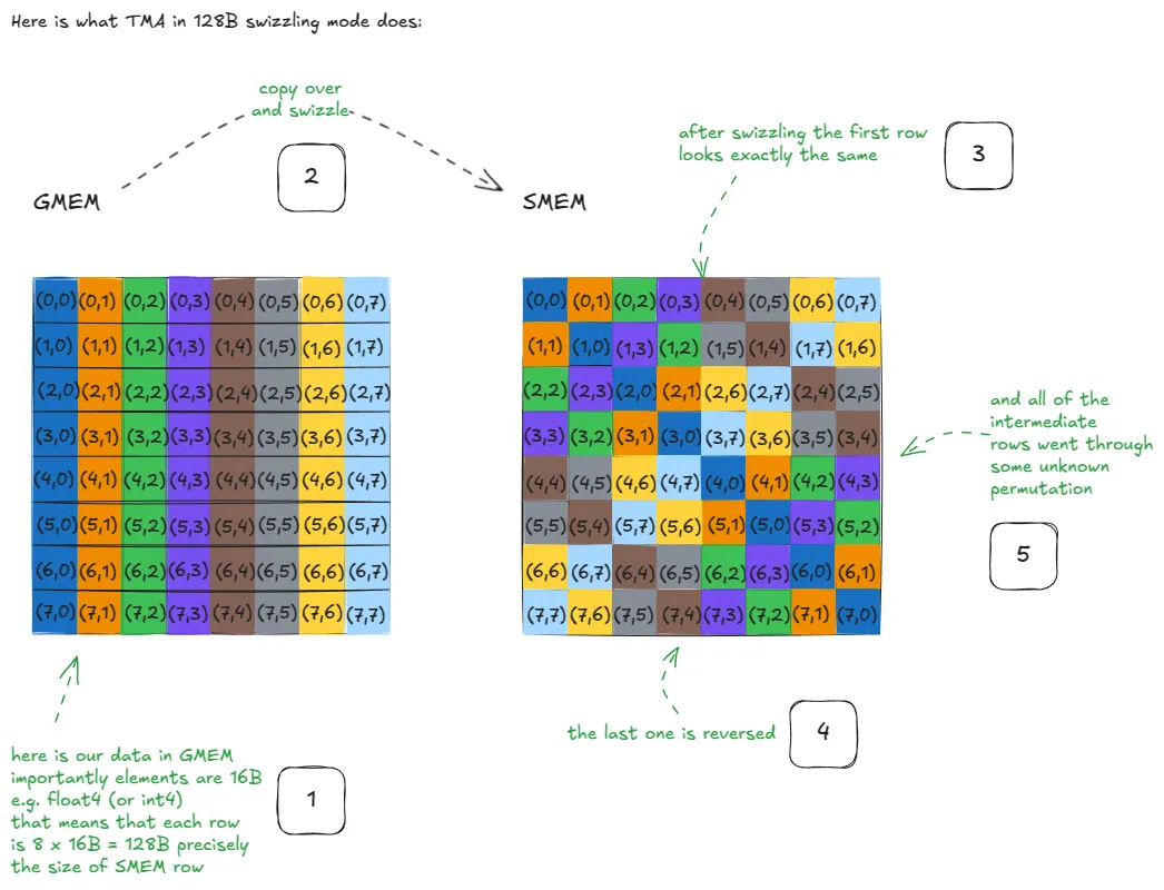
Additionally, we won't need to manually handle padding to avoid SMEM Bank Conflicts like we did before. The hardware automatically applies what’s known as Swizzling. This layout is complex to code by hand, so fortunately, NVIDIA implemented these patterns directly into the TMA. All we need to know is that bank conflicts are essentially handled for us "for free". For more details on the "how" behind the swizzling patterns, Aleksa's post goes into great depth. Here is the figure he used to showcase what a swizzled copy into SMEM looks like at a high level:
To use the TMA, we need to do three main steps:
- Construct tensor maps for our matrices
A&B(On the host). - Trigger TMA operations from the kernel (usually issued by just a single thread in the block).
- Synchronise using specialised Shared Memory barriers.
Tensor Maps
A Tensor Map is a hardware-interpretable descriptor. It describes the shape, layout, and stride of a tensor in memory, allowing the TMA to move entire multi-dimensional tiles without any thread-level address computation.
Unlike earlier kernels, we don't pass raw pointers like const float* A as kernel arguments. Instead, we pass pointers to CUtensorMap descriptors. This is a CUDA Driver defined structure that encodes the full metadata of the matrix (its shape, strides, and its swizzle pattern, allowing the hardware to fetch tiles directly.)
To create these maps, we use the cuTensorMapEncodeTiled function from the CUDA Driver API
 These are the different components that make up the CUDA software platform, and understanding them is important to see what must be called from the host and what is permissible from the device.
At the bottom of the stack sits the CUDA Driver API. It provides the most fine-grained control over the GPU, but is also more verbose and complex. Low-level operations such as tensor map creation are exposed explicitly at this level.
On top of the Driver API sits the CUDA Runtime API, which wraps much of this functionality and offers a higher-level interface. For example, cudaMalloc in the runtime API is a thin wrapper around the driver API’s cuMemAlloc.
Built on top of both APIs are CUDA libraries that provide highly optimised kernels for general and domain-specific workloads, such as cuBLAS for linear algebra and cuDNN for deep neural networks. In practice, most code uses the runtime API, but some Hopper features, such as TMA tensor maps, are currently only exposed through the CUDA Driver API.
. This function takes our description of the matrix and packs it into a 128B hardware descriptor that the TMA engine understands. Because the TMA hardware is so specialised, this 128B object must be aligned to a 128B boundary in memory, or the hardware won't even be able to read it!
The process looks like this:
- Allocate memory for the tensor map on the device using
cudaMalloc. - Encode the map on the Host (CPU) using the Driver API.
- Copy the map from Host to Device using
cudaMemcpy.
In the following code snippet, we perform these steps as follows:
template <const uint BlockMajorSize, const uint BlockMinorSize>
__host__ static inline CUtensorMap *
create_and_allocate_tensor_map(bf16 *tensor_ptr, uint blocks_height, uint blocks_width) {
    CUtensorMap *tensor_map;
    // Allocate device memory for the tensor map descriptor.
    CUDA_CHECK(cudaMalloc((void **)&tensor_map, sizeof(CUtensorMap)));
    // Register the tensorMap in our device memory pointers
    // resources.add_device_ptr(tensor_map);
    // Create on host
    CUtensorMap tensor_map_host;
    create_tensor_map<BlockMajorSize, BlockMinorSize>(&tensor_map_host, tensor_ptr, blocks_height, blocks_width);
    // Copy descriptor to device
    CUDA_CHECK(cudaMemcpy(tensor_map, &tensor_map_host, sizeof(CUtensorMap), cudaMemcpyHostToDevice));
    return tensor_map;
}
And the function which encodes the tensor's metadata and actually creates the tensor map looks like this:
template <const uint BlockMajorSize, const uint BlockMinorSize>
void create_tensor_map(CUtensorMap *tensor_map, bf16 *tensor_ptr, uint blocks_height, uint blocks_width) {
    // Starting address of memory region described by tensor (casting to void
    // as the tensor map descriptor is type-agnostic.)
    void *gmem_address = static_cast<void *>(tensor_ptr);
    uint num_tiles_major = blocks_height;
    uint num_tiles_minor = blocks_width;
    // full size of the tensor in global memory (API expects the 5D supported
    // tensor ranks to be defined)
    uint64_t global_dim[5] = {
        static_cast<uint64_t>(BlockMinorSize * num_tiles_minor),
        static_cast<uint64_t>(BlockMajorSize * num_tiles_major),
        1, 1, 1};
    // Define the tensor strides (in bytes) along each of the tensor ranks dims - 1
    uint64_t global_strides[5] = {
        sizeof(bf16),
        sizeof(bf16) * BlockMinorSize * num_tiles_minor,
        0, 0, 0};
    // Define the shape of the "box_size" -> the tile shapes a TMA ops will load
    uint32_t box_dim[5] = {
        static_cast<uint32_t>(BlockMinorSize),
        static_cast<uint32_t>(BlockMajorSize),
        1, 1, 1};
    uint32_t elem_strides[5] = {1, 1, 1, 1, 1};
    // Create tensor map
    CU_CHECK(cuTensorMapEncodeTiled(
        tensor_map, CU_TENSOR_MAP_DATA_TYPE_BFLOAT16, 2, gmem_address,
        global_dim, global_strides + 1, box_dim, elem_strides,
        CU_TENSOR_MAP_INTERLEAVE_NONE, CU_TENSOR_MAP_SWIZZLE_128B,
        CU_TENSOR_MAP_L2_PROMOTION_NONE, CU_TENSOR_MAP_FLOAT_OOB_FILL_NONE));
}
Next, let’s talk about the WGMMA instructions. WGMMA instructions don’t directly use raw byte addresses the way normal loads and stores do, as we did in all previous kernels. Instead, they take a packed 64-bit matrix descriptor that tells the hardware where the matrix lives in shared memory and how it is laid out.
The format of the matrix descriptor is described in the docs as follows:
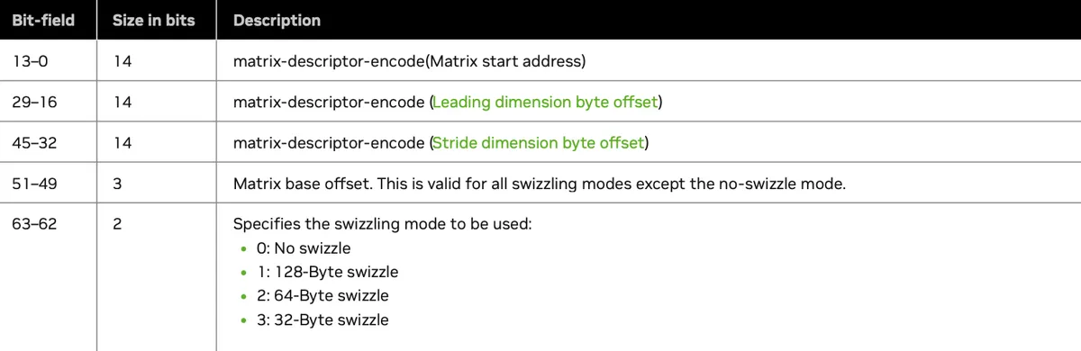
Originally, addresses are byte addresses. For example, an address at 16384 bytes corresponds to 0x4000 in hexadecimal. If the descriptor were to store raw byte addresses directly, it would very quickly run out of bits and severely limit the addressable range.
Instead, the hardware takes advantage of a key property: SMEM operands used by WGMMA are always at least 16B aligned. This means the lowest 4 bits of any valid address are always zero and carry no useful information.
So rather than storing byte addresses, the descriptor stores addresses in units of 16B. This same encoding is applied not only to the base address, but also to the leading dimension and stride offsets, as we can see in the table above. By doing this, the descriptor can represent much larger SMEM regions while still fitting all required metadata into a single 64-bit value that the hardware can efficiently broadcast and decode across the entire warp group.
A conceptual example of how this encoding happens looks like this:
![matrix-desc-encoding]](https://bear-images.sfo2.cdn.digitaloceanspaces.com/testing-inf1/excalidraw-52.svg)
The encoding logic and descriptor construction must run on the device, since WGMMA matrix descriptors are built inside the kernel. We construct the matrix descriptor in the make_smem_descriptor function.
We also will first need to convert the generic pointer bf16* into a shared-memory address using __cvta_generic_to_shared before encoding it. This step is subtle but essential. WGMMA is not a C++ abstraction, but a low-level hardware instruction that expects a SMEM byte address in a very specific format. A regular CUDA C++ pointer does not explicitly encode its address space (i.e Global, Shared etc.), so we cannot directly use or encode it. Instead, we must first convert the pointer into a concrete SMEM address that the hardware understands, and only then compress and pack it into the matrix descriptor
CUDA C++ pointers are generic, meaning they can refer to objects in global or shared memory without explicitly encoding the address space. This abstraction works well for normal C++ loads and stores, but it breaks down when interacting directly with PTX instructions or hardware interfaces such as WGMMA. These interfaces require addresses that explicitly refer to a specific memory space. To bridge this gap, CUDA provides address-space conversion intrinsics such as __cvta_generic_to_shared, which convert a generic pointer into a shared-memory address that can be consumed by PTX instructions and hardware descriptors.
. The code for both functions look like this:
__device__ static inline uint64_t matrix_descriptor_encode(uint64_t x) {
    return ((x) & 0x3FFFF) >> 4;
}

__device__ uint64_t make_smem_desc(bf16* ptr) {
    uint32_t address = static_cast<uint32_t>(__cvta_generic_to_shared(ptr));
    // Initialise an empty 64 bit descriptor
    uint64_t desc = 0x0000000000000000;
    // bitwise OR
    // sets bits [13:0] encoded matrix start address
    desc |= matrix_descriptor_encode(address);
    // sets bits [29:16] leading dimension byte offset
    desc |= matrix_descriptor_encode(static_cast<uint64_t>(16)) << 16;
    // sets bits [45: 32] stride dimension byte offset
    desc |= matrix_descriptor_encode(static_cast<uint64_t>(1024)) << 32;
    // sets bits [62: 63] swizzle mode
    desc |= 1llu << 62;
    return desc;
}
In the make_smem_desc function, we first initialise an empty 64-bit descriptor that we will eventually return. We then fill this descriptor field by field according to the matrix descriptor layout above.
First, we encode the matrix start address and place it in bits [13:0] of the descriptor. This represents the base address of the matrix in shared memory, encoded in units of 16 bytes. Next, we encode the leading dimension byte offset and place it in bits [29:16]. This describes how far (in bytes) the hardware must move to advance along the leading dimension of the matrix.
The third field is the stride dimension byte offset, which is placed in bits [45:32]. As described in the documentation:
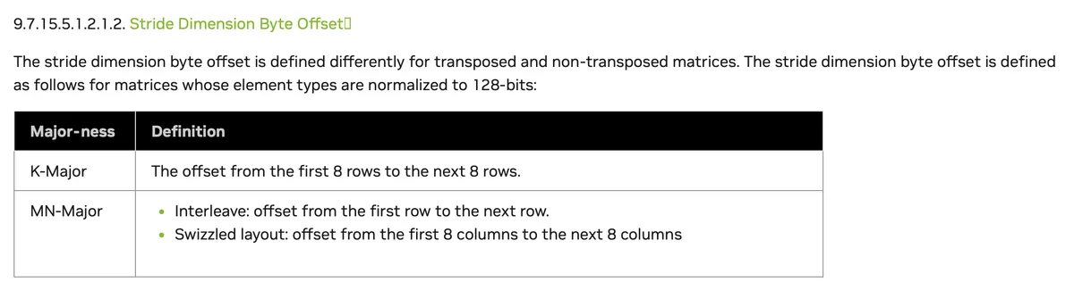
Conceptually, this field answers the question:
“How far (in bytes) do we move to go from columns 0–7 to columns 8–15 (along the K dimension)?”
We haven’t introduced our exact tile shapes yet, but spoiler alert: sharedA will be a 64 × 64 matrix. Each column contains 64 bf16 elements, and each bf16 is 2 bytes, so a single column is 128 bytes wide. To jump 8 columns along K, we therefore need: 8 × 128 bytes = 1024 bytes. So we encode the stride dimension byte offset as 1024.
Finally, the last field specifies the swizzling mode, stored in bits [63:62]. Since we are using 128-byte swizzling, we set this field to 1. This field does not go through the encoding function, as it is a fixed enumerated value rather than a byte offset.
Kernel Structure
Now, let’s get to the main part and talk about the kernel itself and start putting everything together. With the only caveat that we will not go into the detail of how we define the WGMMA instruction now. We will leave it as a black box for now, just for the sake of the narrative, and we’ll come back to it in detail after.
Before looking at any code for the kernel I would like to start first by laying out the high level kernel flow structure and showing visually how that would look like.
- We start with the same block tiling strategy we’ve used throughout this series. This is our GMEM view and the highest level of abstraction.
- During each iteration over the K dimension, we use the TMA to load full 2D tiles of
AandBfrom GMEM into SMEM. - The warp group then issues the WGMMA operations on these tiles. In our kernel, that means issuing four
m64n64k16WGMMA instructions perKiteration. - This repeats until all
Ktiles have been processed, with results accumulated in registers. - At the end, each thread stores its register fragment back to global memory, producing the final output tile in
C

As we can see, during each tensor core MMA we take the outer product of a subtile of sharedA with a subtile of sharedB to update an accumulator tile of size TILE_SIZE_M(64) × TILE_SIZE_N(64).
The operand placement rules tell us:
sharedAcan live in registers or shared memory.sharedBmust live in shared memory.- The accumulator
Dmust live in registers (C's tile) in the drawing.
Clearly, no single thread can hold a full 64 × 64 accumulator. Instead, the accumulator is distributed across the entire warp group. In our case, the warp group consists of 128 threads, and all 128 threads cooperate to execute each m64n64k16 WGMMA instruction. Within a single K-iteration, the warp group issues multiple WGMMA instructions back-to-back, each operating on a different slice of the K dimension (2.1, 2.2, etc) and accumulating into the same per-thread registers. Together, these instructions build up the full 64 × 64 output tile.
This layout is not something we choose manually. It is fixed by the hardware and described in section 9.7.15.5.1.1. of the PTX documentation, which defines the register fragment layout for m64n64k16 and explains how the accumulator tile is distributed across the warp group.
In the code, this shows up when we initialise the per-thread accumulator registers:
// Initialise thread's accumilator
// d[4][8] = 32 floats per thread
float d[WGMMA_N / 16][8];
memset(d, 0, sizeof(d));
Each thread owns exactly 32 floating-point accumulator values, which together form that thread’s fragment of the overall 64 × 64 output tile. During each WGMMA step, these registers are updated in place. Next, we create two SMEM barriers and initialise them to synchronise writes into sharedA and sharedB. Both barriers are initialised with all 128 threads in the warp group.
// SMEM barriers for A and B
__shared__ barrier barA;
__shared__ barrier barB;

if (threadIdx.x == 0) {
    init(&barA, blockDim.x);
    init(&barB, blockDim.x);
    cde::fence_proxy_async_shared_cta();
}
__syncthreads();
Notice, even though we use the cuda::barrier<cuda::thread_scope_block> API (barrier was aliased) , we are still issuing a single __syncthreads(). The reason for this is due to a bootstrapping problem.
As stated in the docs, before threads can start synchronising using these barriers, the barrier must first be initialised from within the kernel. But, how do threads synchronise in order to initialise the barrier in the first place?
This is why we still use __syncthreads(). We briefly fall back to an older synchronisation primitive just once, to ensure all threads are synchronised after the barrier has been initialised (since we already seen in earlier kernels __syncthreads() doesn't need to be initialised). After this one-time bootstrap, we can safely use cuda::barrier normally for the rest of the kernel.
We then start the outer loop iterating over num_blocks_k (The shared dim), just like in all our previous kernels, and begin issuing bulk loads using the TMA:
barrier::arrival_token tokenA, tokenB;
for (int block_k_iter = 0; block_k_iter < num_blocks_k; block_k_iter++) {
    // Async loads (Only 1 thread launches the TMA op)
    if (threadIdx.x == 0) {
        // Thread 0 launches async bulk tensor copy operations for both matrices
        cde::cp_async_bulk_tensor_2d_global_to_shared(&sharedA[0], tensorMapA, block_k_iter * TILE_SIZE_K, num_block_m * TILE_SIZE_M, barA);
        // Signal barrier and wait for both loads to complete
        tokenA = cuda::device::barrier_arrive_tx(barA, 1, sizeof(sharedA));
        cde::cp_async_bulk_tensor_2d_global_to_shared(&sharedB[0], tensorMapB, block_k_iter * TILE_SIZE_K, num_block_n * TILE_SIZE_N, barB);
        tokenB = cuda::device::barrier_arrive_tx(barB, 1, sizeof(sharedB));
    }
    else {
        // Other threads arrive at barrier to synchronise data loads
        tokenA = barA.arrive();
        tokenB = barB.arrive();
    }
    // All threads wait for async loads to complete
    barA.wait(std::move(tokenA));
    barB.wait(std::move(tokenB));
    __syncthreads();
}
During each iteration over the K dimension, a single thread in the block (thread 0) is responsible for launching the TMA loads for both matrices A and B using cp_async_bulk_tensor_2d_global_to_shared. These instructions enqueue asynchronous bulk copies that move full 2D tiles from GMEM into SMEM based on the tensor maps we constructed earlier. Immediately after issuing each copy, thread 0 calls barrier_arrive_tx, which does two things: it signals its arrival at the barrier, and it informs the barrier of how many bytes are expected to be written by the asynchronous copy. All other threads in the block simply call bar.arrive(), contributing their arrival without attaching any data transfer. Finally, all threads wait on the barrier using bar.wait(token) (See the docs for this one). This wait only completes once all threads in the block have arrived and the TMA engine has finished writing the full tile into SMEM.
At that point, we are guaranteed that the SMEM tiles are fully populated and visible to all threads, and it is safe to proceed to the WGMMA compute phase. This is where the warp group executes the WGMMA instructions that actually perform the MMAs. The compute phase follows these steps:
- Fence the warp group state: We first issue
wgmma.fence.sync.aligned. Conceptually, this indicates that all relevant register and SMEM writes across the warp group are complete and visible, and that the warp group is ready to begin issuing WGMMA instructions. - Issue the WGMMA operations: We then sequentially issue multiple asynchronous WGMMA operations using
wgmma.mma_async. In the code, each call towgmma64is a thin wrapper around a singlewgmma.mma_async.m64n64k16instruction, which we intentionally treat as a black box for now and will look into in detail next. Each WGMMA instruction computes a64 × 64 × 16matrix multiply and accumulates into the same per-thread accumulator registers. Across the four calls, we are effectively stepping through different slices of theKdimension while accumulating into the same64 × 64output tile. Thesewgmma.mma_asyncinstructions are asynchronous: issuing them does not imply immediate completion. Instead, they are queued by the hardware for later execution. - Commit the WGMMA group: Create a wgmma-group and commit all the prior outstanding
wgmma.mma_asyncoperations into the group, by usingwgmma.commit_groupoperation. - Wait for completion of the required wgmma-group
wgmma.wait_group. - Proceed once complete: Once the WGMMA group completes, all issued
wgmma.mma_asyncoperations have been executed, and the accumulated results are safely available in registers. At this point, the kernel can either move on to the next K tile or proceed to the store phase.
// Compute phase using WGMMA tensor cores
warpgroup_arrive(); // asm volatile("wgmma.fence.sync.aligned;\n" ::: "memory");
wgmma64<1, 1, 1, 0, 0>(d, &sharedA[0], &sharedB[0]);
wgmma64<1, 1, 1, 0, 0>(d, &sharedA[WGMMA_K], &sharedB[WGMMA_K]);
wgmma64<1, 1, 1, 0, 0>(d, &sharedA[2 * WGMMA_K], &sharedB[2 * WGMMA_K]);
wgmma64<1, 1, 1, 0, 0>(d, &sharedA[3 * WGMMA_K], &sharedB[3 * WGMMA_K]);
warpgroup_commit_batch(); // asm volatile("wgmma.commit_group.sync.aligned;\n" ::: "memory");
warpgroup_wait<0>();      // asm volatile("wgmma.wait_group.sync.aligned %0;\n" ::"n"(N) : "memory");
The last missing piece is actually the WGMMA instruction itself. Above, I intentionally focused on the overall kernel structure first: how tiles are loaded with TMA, how synchronisation works, and how the compute phase is organised. We already saw the wgmma64 function being called during the compute phase, but so far we have treated it as a black box. Now we can finally open it up.
The wgmma64 function is a thin wrapper around the inline PTX instruction: wgmma.mma_async.m64n64k16.f32.bf16.bf16. Its entire shape and signature are dictated by the hardware interface:
template <int ScaleD, int ScaleA, int ScaleB, int TransA, int TransB>
__device__ void wgmma64(float d[4][8], bf16 *sharedA, bf16 *sharedB)
{
    uint64_t desc_a = make_smem_desc(&sharedA[0]);
    uint64_t desc_b = make_smem_desc(&sharedB[0]);
Each call begins by constructing two matrix descriptors, one for matrix A and one for matrix B. These descriptors encode where the matrices live in SMEM and how they are laid out. As discussed earlier, WGMMA does not accept raw pointers; it consumes these packed 64-bit descriptors instead.
The core of the function is the inline PTX block:
    asm volatile(
        "{\n"
        "wgmma.mma_async.sync.aligned.m64n64k16.f32.bf16.bf16 "
        "{%0,   %1,   %2,   %3,   %4,   %5,   %6,   %7,   "
        " %8,   %9,   %10,  %11,  %12,  %13,  %14,  %15,  "
        " %16,  %17,  %18,  %19,  %20,  %21,  %22,  %23,  "
        " %24,  %25,  %26,  %27,  %28,  %29,  %30,  %31},""
        " %32,"
        " %33,"
        " %34, %35, %36, %37, %38;\n"
        "}\n"
        : "+f"(d[0][0]), "+f"(d[0][1]), "+f"(d[0][2]), "+f"(d[0][3]), "+f"(d[0][4]), "+f"(d[0][5]),
          "+f"(d[0][6]), "+f"(d[0][7]), "+f"(d[1][0]), "+f"(d[1][1]), "+f"(d[1][2]), "+f"(d[1][3]),
          "+f"(d[1][4]), "+f"(d[1][5]), "+f"(d[1][6]), "+f"(d[1][7]), "+f"(d[2][0]), "+f"(d[2][1]),
          "+f"(d[2][2]), "+f"(d[2][3]), "+f"(d[2][4]), "+f"(d[2][5]), "+f"(d[2][6]), "+f"(d[2][7]),
          "+f"(d[3][0]), "+f"(d[3][1]), "+f"(d[3][2]), "+f"(d[3][3]), "+f"(d[3][4]), "+f"(d[3][5]),
          "+f"(d[3][6]), "+f"(d[3][7])
        : "l"(desc_a), "l"(desc_b), "n"(int32_t(ScaleD)), "n"(int32_t(ScaleA)),
          "n"(int32_t(ScaleB)), "n"(int32_t(TransA)), "n"(int32_t(TransB)));
The long list {%0 … %31} corresponds to the accumulator registers owned by the calling thread. These are both inputs and outputs, which is why they are marked with "+f" in the operand list. Each WGMMA instruction reads the current values from these registers, performs the MMA, and writes the updated results back into the same registers.
The next two operands, %32 and %33, are the matrix descriptors for A and B in SMEM. The final operands encode scaling and transpose flags, which are template parameters so they can be compile-time constants and directly embedded into the instruction.
Once all WGMMA instructions for a given K-iteration have been issued and completed, the accumulator registers contain the final results for the output tile. The last step is to write these values back to global memory.
I’ll first show the code snippet responsible for the stores. Then, I’ll revisit the full register fragment layout for the accumulator D (which corresponds to C in our code), as defined in the documentation. However, instead of trying to interpret the entire warp-group layout at once, I’ll explain it by focusing on a single thread (specifically thread 0). By understanding how one thread’s register fragments map to output elements, the full layout naturally falls into place.
for (int m_it = 0; m_it < TILE_SIZE_M / WGMMA_M; ++m_it) {
    for (int n_it = 0; n_it < TILE_SIZE_N / WGMMA_N; ++n_it) {
        for (int w = 0; w < WGMMA_N / 16; ++w) { // w = {0, 1, 2, 3}
            // (16 * w) selects the base col of the 16 col block
            int col = 16 * w + 2 * (tid % 4);
            #define IDX(i, j) ((j + n_it * WGMMA_N) * M + ((i) + m_it * WGMMA_M))
            // Apply alpha scaling to accumulator results and add beta*C
            block_C[IDX(row, col)] = __float2bfloat16(alpha * d[w][0] + beta * __bfloat162float(block_C[IDX(row, col)]));
            block_C[IDX(row, col + 1)] = __float2bfloat16(alpha * d[w][1] + beta * __bfloat162float(block_C[IDX(row, col + 1)]));
            block_C[IDX(row + 8, col)] = __float2bfloat16(alpha * d[w][2] + beta * __bfloat162float(block_C[IDX(row + 8, col)]));
            block_C[IDX(row + 8, col + 1)] = __float2bfloat16(alpha * d[w][3] + beta * __bfloat162float(block_C[IDX(row + 8, col + 1)]));
            block_C[IDX(row, col + 8)] = __float2bfloat16(alpha * d[w][4] + beta * __bfloat162float(block_C[IDX(row, col + 8)]));
            block_C[IDX(row, col + 9)] = __float2bfloat16(alpha * d[w][5] + beta * __bfloat162float(block_C[IDX(row, col + 9)]));
            block_C[IDX(row + 8, col + 8)] = __float2bfloat16(alpha * d[w][6] + beta * __bfloat162float(block_C[IDX(row + 8, col + 8)]));
            block_C[IDX(row + 8, col + 9)] = __float2bfloat16(alpha * d[w][7] + beta * __bfloat162float(block_C[IDX(row + 8, col + 9)]));
            #undef IDX
        }
    }
}
Here, each thread computes the row index it is responsible for based on its warp and lane. The nested loops that follow iterate over the logical tiles in the M and N dimensions, and over the internal fragment structure. For each iteration, the thread writes out the corresponding elements from its accumulator registers into the correct positions in GMEM.
This is how the register fragment layout looks like for all threads, focusing on thread 0 only as an example:

At this point, we have walked through the entire kernel end-to-end, both from a code perspective and from the underlying hardware execution model. With all the pieces in place, the next step is to benchmark the kernel and look at the performance results.
We achieve throughput of 280.4 TFLOP/s, a HUGE improvement from our last kernel, which only achieved 41.4 for the full FP32 path and 31.5 for the mixed precision. Simply a different ball game.
Performance compared to the full FP32 cuBLAS benchmark is now ~544%, but obviously from now on this comparison isn't "fair" as this cuBLAS version doesn't use tensor cores; I just wanted to put them together to see the big difference.
Our real benchmark from now on is the cuBLAS with bf16 and tensor cores activated. For that, we achieve 37.8%. (Which btw, even though in earlier kernels I reported the FP32 comparative relative performances, I also tested them out in mixed precision compared to the cuBLAS with tensor cores, and the warp tiling achieved only 4.3%, so technically we jumped from 4.3% to 37.8%, almost a 9x improvement.
Kernel 8: Exploring WGMMA Shapes
So far, we have only experimented with a single WGMMA shape: m64n64k16. Unlike traditional CUDA kernels, where we are free to experiment with arbitrary tile sizes as long as the math works out, tensor core MMA operations are much more constrained. NVIDIA only supports a limited, fixed set of matrix shapes for the operands A, B, and the accumulator C, as documented in the PTX ISA specification (See table below).
Each of these supported MMA shapes corresponds to a specific hardware instruction and determines the size of the output tile produced by a single WGMMA operation. Some shapes naturally produce larger accumulator tiles, while others result in smaller ones. This directly affects how much work a warp group performs per instruction and, consequently, how the kernel needs to be structured around it.
Naturally, if we can choose an MMA shape that allows each warp group to produce more output elements per instruction, we can expect higher performance, since more arithmetic work is performed per issued WGMMA. Of course, this only holds as long as we are not limited by other factors such as register pressure which in turn could lead to reduced occupancy.
For this kernel, our goal is to explore different WGMMA configurations and evaluate which ones are the best fit for the H100 architecture. Rather than exhaustively testing every possible option, we will focus on a small subset of bf16-supported shapes and compare their impact on performance.
Below are the bf16 WGMMA shapes supported by the hardware. From this list, we will select a few representative candidates to experiment with and analyse further.
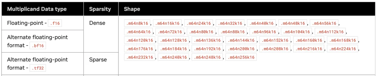
Only the
Ndimension changes.Mis fixed at 64,Kis fixed at 16 for these bf16 dense shapes.
Visually, this kernel is almost identical to the previous one. The key difference is the introduction of an outer loop that allows us to cover a larger TILE_SIZE_M. To make this concrete, we can imagine increasing TILE_SIZE_M from 64 to 128 and see how the kernel now iterates over two M-tiles instead of one within a single block.

With TILE_SIZE_M = 128, TILE_SIZE_N = 128, and TILE_SIZE_K = 64, and knowing from the WGMMA shape table that WGMMA_K is fixed at 16, the K dimension is still partitioned into four vertical panels, exactly as in the previous kernel.
What changes is theTILE_SIZE_M dimension. The WGMMA shape table tells us that WGMMA_M is fixed at 64, so a single WGMMA operation can only produce 64 rows of output at a time. Because our block now covers 128 rows, we must explicitly loop over the TILE_SIZE_M dimension and invoke WGMMA twice, once for the first 64 rows and once for the second 64 rows, in order to cover the full output tile.
For this kernel, the structure is therefore:
- Pick
WGMMA_N=TILE_SIZE_Nwhen supported, to cover the full block width in one instruction. - Loop over
m_itto coverTILE_SIZE_M. - Loop over
k_itto coverTILE_SIZE_K.
Otherwise, the kernel remains logically the same in terms of TMA loads, SMEM layout, and stores; the primary difference lies in how the compute phase is structured around the WGMMA instruction shape. Below for example is how the new kernel's compute phase would look like if we used the m64n128k16 shape and increased TILE_SIZE_M = 128:
The core of this kernel is therefore the compute phase, which looks like this:
// 2. Compute phase using WGMMA tensor cores instructions
warpgroup_arrive();
// Outer loop over TILE_SIZE_M in WGMMA_M steps
// If we have two warp groups, we let each work on a different partition of TILE_SIZE_M
// @example:
#pragma unroll
for (int m_iter = 0; m_iter < rows_per_warp_group / WGMMA_M; m_iter++) {
    bf16* sharedA_wgmma_tile_base = sharedA + ((warp_group_idx * rows_per_warp_group) + (m_iter * WGMMA_M)) * TILE_SIZE_K;
    // Inner loop iterating over TILE_SIZE_K in WGMMA_K steps
    #pragma unroll
    for (int k_iter = 0; k_iter < TILE_SIZE_K / WGMMA_K; k_iter++) {
        wgmma<WGMMA_N, 1, 1, 1, 0, 0>(d[m_iter], &sharedA_wgmma_tile_base[k_iter * WGMMA_K], &sharedB[k_iter * WGMMA_K]);
    }
}
warpgroup_commit_batch(); // asm volatile("wgmma.commit_group.sync.aligned;\n" ::: "memory");
warpgroup_wait<0>(); // asm volatile("wgmma.wait_group.sync.aligned %0;\n" ::"n"(N) : "memory");
}
| WGMMA_N | TFLOP/s | Perf. relative to cuBLAS % |
|---|---|---|
| 32 | 230.2 | 31.7% |
| 128 | 407.7 | 56.9% |
| 256 | 70.3 | 9.7% |
After experimenting with a few different WGMMA_N shapes, we see the expected behaviour that we alluded to earlier. A value of 128 gives the best balance between instruction efficiency and memory reuse, 64 comes close behind and matches our previous kernel, 32 underutilises the tensor cores, and 256 explodes register pressure, collapsing performance. Overall, this gives us another ~1.5× improvement over the last kernel, and we now reach 56.9% of cuBLAS performance, meaning we are roughly halfway there.
Profiling
At the start of the previous kernel’s section we asked the question:
“How do we place the required matrix tiles into shared memory in the exact format that WGMMA expects, and do so quickly enough that the tensor cores never sit idle?”
We answered the first part, but given the profiling results from this kernel, we clearly have not answered the second question yet.
First, looking at the compute throughput breakdown in the SoL section, we see that the tensor pipeline is significantly underutilised. The metric SM: Pipe Tensor Cycles Active reaches only 51.17% of its peak sustained rate, indicating that the tensor MMA units are idle for nearly half of the kernel’s execution time. At the same time, none of the memory systems are close to their theoretical peak, which strongly suggests that the kernel is scheduling bound rather than memory bound. To understand why, we now turn to the scheduler and warp statistics.
Looking at the scheduler statistics, we find that:
- Active warps per scheduler = 2.94
- Eligible warps per scheduler = 0.19
- Issued warps per scheduler = 0.17
This tells us that although several warps are resident on each scheduler, almost none of them are ready to run at any given cycle. In other words, the scheduler frequently wants to issue work but has no eligible warps to choose from. This is, by definition, a scheduling and dependency problem.
Initially, I tried increasing NUM_THREADS to 256 so that each block would contain two warp groups. The intuition was that this would increase occupancy and the number of active warps, helping to hide latency. While both occupancy and active warps did increase, performance did not improve and in fact became slightly worse. The reason is that occupancy alone does not produce eligible warps. In this case, eligible warps per scheduler only increased marginally from 0.19 to 0.23, which is far too small to meaningfully change scheduling behaviour.
🔎 Here are the scheduler and warp statistics of the 128-thread kernel (baseline) and the 256-thread kernel (current) compared with one another showing that active warps did increase, but didn't lead to any improvements as warps still had similar stalling issues (Please zoom in to read metrics clearly):
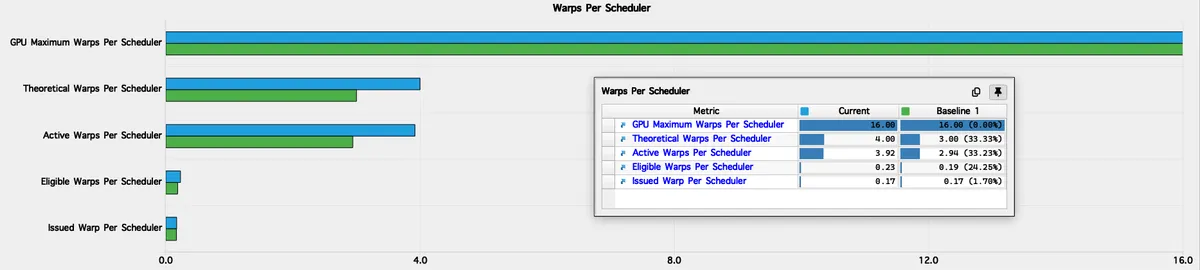
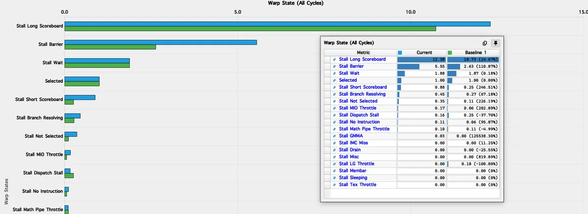
Increasing the number of threads can raise occupancy, but if all of those warps are still blocked on barriers, waits, or dependency chains, then the scheduler still has very little useful work to issue. This motivates a closer look at the warp state statistics for the original 128 thread kernel.
The dominant stall reason is Long Scoreboard at 10.73, meaning that warps are frequently blocked on outstanding dependencies flowing through the execution and memory pipelines. In this kernel, the primary source of these dependencies is the accumulation loop itself. Each WGMMA instruction reads from and writes to the same accumulator registers, so successive WGMMA operations are inherently dependent. This serial dependency within the accumulation loop is fundamental to the GEMM algorithm and remains unchanged.
Barrier and Wait stalls are also significant. Every iteration over the K dimension follows the same strictly serial pattern: TMA loads are issued, the kernel waits for those loads to complete, the CTA is synchronised, WGMMA compute is executed, and finally all outstanding WGMMA work is drained before the next iteration begins. With so few eligible warps per scheduler, none of these latencies can be hidden, leaving the tensor pipeline idle for a substantial fraction of execution time.
In effect, the kernel exhibits large pipeline bubbles at the iteration level. During the WGMMA compute phase, the memory system is idle. During the TMA load and synchronisation phases, the tensor cores are idle. Because this pattern repeats identically for all 128 K iterations, these idle periods accumulate into a large loss of efficiency, which directly explains the low tensor pipe utilisation observed in profiling.
Below are the locations in the code where these stalls arise:
// TMA launch on one thread
if (threadIdx.x == 0) {
    cde::cp_async_bulk_tensor_2d_global_to_shared(..., barA);
    tokenA = cuda::device::barrier_arrive_tx(barA, 1, sizeof(s.A));
    cde::cp_async_bulk_tensor_2d_global_to_shared(..., barB);
    tokenB = cuda::device::barrier_arrive_tx(barB, 1, sizeof(s.B));
}
else {
    tokenA = barA.arrive();
    tokenB = barB.arrive();
}
// Stall Barrier: arrival skew (other warps reach arrive/wait earlier than thread 0)
// Stall Wait: arrive_tx ties barrier completion to async copy bytes landing

barA.wait(std::move(tokenA));
barB.wait(std::move(tokenB));
// Stall Wait: waiting for TMA transaction completion (bytes written to SMEM)
// Stall Barrier: waiting for all warps to arrive at the barrier phase

__syncthreads();
// Stall Barrier: explicit CTA barrier each K-iteration (often redundant here)

for (int k_iter = 0; k_iter < TILE_SIZE_K / WGMMA_K; k_iter++) {
    wgmma(...)(d[m_iter], ...);
    // Stall Long Scoreboard: dependency chain on d[m_iter] registers
    // each WGMMA reads+writes d, next WGMMA needs updated d
}

warpgroup_wait<0>();
// Stall Wait: explicit drain of all WGMMA work before next iteration
Visually, this is each thread's pipeline:

Kernel 9: Asynchronous Producer–Consumer Pipeline with Epilogue Shared Memory Staging
Given the pipeline serialisation identified in the previous kernel, the next step is to restructure the kernel into a producer-consumer pattern. In this design, one warp group acts as a producer, whose primary responsibility is to issue TMA loads, while the remaining warp group(s) act as consumers, responsible for executing the tensor core compute using WGMMA.
Crucially, these roles operate in parallel. While the consumer warp group is executing WGMMA on the current K tile, the producer warp group can already be issuing asynchronous TMA loads for the next tile. This leverages the fact that TMA transfers run independently of the tensor core pipeline.
The goal of this kernel is not to eliminate the serial accumulation dependency inside WGMMA, which is fundamental to GEMM and cannot be removed. Instead, the objective is to hide load and synchronisation latency across K iterations by overlapping TMA loads with tensor core compute. By doing so, we aim to (1) reduce pipeline bubbles, (2) increase tensor core pipe utilisation, and (3) improve scheduler behaviour by increasing the number of eligible warps and (4) reducing long scoreboard stalls.
Before diving into the implementation, the figure below shows the execution model we are aiming for visually:

The kernel's core look like this:
#pragma nv_diag_suppress static_var_with_dynamic_init
__shared__ barrier full[NUM_STAGES];  // Signals data is ready
__shared__ barrier empty[NUM_STAGES]; // Signals slot is available

if (threadIdx.x == 0) {
    for (int i = 0; i < NUM_STAGES; i++) {
        init(&full[i], num_consumer_groups * 128 + 1); // consumers + producer thread 0
        init(&empty[i], num_consumer_groups * 128 + 1);
    }
    cde::fence_proxy_async_shared_cta();
}
__syncthreads();

if (is_producer) {
    // Producer warp group: Issues TMA loads
    if (threadIdx.x == 0) {
        // Fill the pipeline
        for (int stage = 0; stage < NUM_STAGES && stage < num_blocks_k; stage++) {
            int block_k_iter = stage;

            // Wait for empty slot (initially all are empty, so this passes immediately)
            empty[stage].wait(empty[stage].arrive());

            // Get pointers for this stage in the flat arrays
            bf16* A_stage = s.A + (stage * A_stage_size);
            bf16* B_stage = s.B + (stage * B_stage_size);

            // TMA loads for A and B
            cde::cp_async_bulk_tensor_2d_global_to_shared(A_stage, tensorMapA, block_k_iter * TILE_SIZE_K, num_block_m * TILE_SIZE_M, full[stage]);
            cde::cp_async_bulk_tensor_2d_global_to_shared(B_stage, tensorMapB, block_k_iter * TILE_SIZE_K, num_block_n * TILE_SIZE_N, full[stage]);

            // Signal data is ready
            barrier::arrival_token token = cuda::device::barrier_arrive_tx(full[stage], 1, A_stage_size * sizeof(bf16) + B_stage_size * sizeof(bf16));
        }

        // Main loop: Continue issuing loads
        for (int block_k_iter = NUM_STAGES; block_k_iter < num_blocks_k; block_k_iter++) {
            int stage = block_k_iter % NUM_STAGES;

            // Wait for this stage to be empty before overwriting
            empty[stage].wait(empty[stage].arrive());

            // Get pointers for this stage in the flat arrays
            bf16* A_stage = s.A + (stage * A_stage_size);
            bf16* B_stage = s.B + (stage * B_stage_size);

            // Issue next TMA loads
            cde::cp_async_bulk_tensor_2d_global_to_shared(A_stage, tensorMapA, block_k_iter * TILE_SIZE_K, num_block_m * TILE_SIZE_M, full[stage]);
            cde::cp_async_bulk_tensor_2d_global_to_shared(B_stage, tensorMapB, block_k_iter * TILE_SIZE_K, num_block_n * TILE_SIZE_N, full[stage]);

            // Signal data is ready
            barrier::arrival_token token = cuda::device::barrier_arrive_tx(full[stage], 1, A_stage_size * sizeof(bf16) + B_stage_size * sizeof(bf16));
        }
    }

} else {
    // Consumer warp groups: Execute WGMMA compute
    // Accumulator registers - declared inside consumer branch only so
    // ptxas doesn't allocate them for the producer warp group
    float d[TILE_SIZE_M / WGMMA_M / num_consumer_groups][WGMMA_N / 16][8];
    memset(d, 0, sizeof(d));

    // Initially signal all empty slots are available
    for (int i = 0; i < NUM_STAGES; i++) {
        barrier::arrival_token token = empty[i].arrive();
    }

    // Main compute loop
    for (int block_k_iter = 0; block_k_iter < num_blocks_k; block_k_iter++) {
        int stage = block_k_iter % NUM_STAGES;

        // Get pointers for this stage in the flat arrays
        bf16* A_stage = s.A + (stage * A_stage_size);
        bf16* B_stage = s.B + (stage * B_stage_size);

        // Wait for data to be ready
        full[stage].arrive_and_wait();

        // Compute phase using WGMMA
        warpgroup_arrive();

        #pragma unroll
        for (int m_iter = 0; m_iter < rows_per_consumer_warp_group / WGMMA_M; m_iter++) {
            bf16* sharedA_wgmma_tile_base = A_stage + ((consumer_warp_group_idx * rows_per_consumer_warp_group) + (m_iter * WGMMA_M)) * TILE_SIZE_K;

            #pragma unroll
            for (int k_iter = 0; k_iter < TILE_SIZE_K / WGMMA_K; k_iter++) {
                wgmma<WGMMA_N, 1, 1, 1, 0, 0>(d[m_iter], &sharedA_wgmma_tile_base[k_iter * WGMMA_K], &B_stage[k_iter * WGMMA_K]);
            }
        }

        warpgroup_commit_batch();
        warpgroup_wait<0>();

        // Signal this slot is now empty and can be reused
        barrier::arrival_token empty_token = empty[stage].arrive();
    }
}
To coordinate the pipeline properly, we allocate two arrays of shared memory barriers per pipeline stage: empty[stage] means “this stage buffer can be written into”, and full[stage] means “this stage buffer now contains valid A and B tiles”. Thread 0 initialises every barrier with the expected participant count and then all threads sync once so the barriers are ready. After that, the producer (again driven by thread 0) first “primes” the pipeline by looping over the first few K tiles, waiting for each stage to be empty, issuing the two TMA loads into that stage’s s.A and s.B slices, then signalling full[stage] using a transaction arrive so consumers can wake when the bytes have landed. Once the pipeline is full, the producer continues in a steady state: for each new K tile it reuses stage = block_k_iter % NUM_STAGES, waits until consumers mark that stage empty, then overwrites it with the next TMA loads and signals full again. Meanwhile, each consumer warpgroup allocates its accumulator fragment d in registers, marks all stages as initially empty (so the producer can start immediately), then runs a K loop where it picks the same cyclic stage, waits on full[stage] until the producer has finished loading that stage, runs the WGMMA microloops over the A subtiles it owns and the B tile for that stage, commits and waits for the WGMMA batch to finish, then marks empty[stage] to hand that stage buffer back to the producer for reuse on the next cycle.
This next visual should make it clearer how the producer and consumers cooperate together:
Debugging
After implementing the kernel, I expected to see the same performance improvement reported by Pranjal's implementation. Our previous kernel had already matched his performance almost exactly, so the comparison was fair. If his kernel showed a large uplift from adding the pipeline, mine should demonstrate similar gains. But it did not. This immediately suggested that either my implementation differed structurally in a way that prevented proper overlap, or something more fundamental was limiting the pipeline's effectiveness. I had reorganised the producer side slightly, splitting the prefill phase and steady state into separate loops and restructuring stage addressing. These changes were semantically correct but diverged from his implementation's structure, making it unclear where the problem originated.
Profiling became key to identifying what went wrong through a series of targeted experiments. You can find all profiling reports in the repo at h100_gemm/profiling_reports/producer-consumer-pipeline
Isolating the Variable
The key insight was to isolate the effect of output scaling independently from any implementation differences. I profiled Pranjal's implementation directly in two configurations:
- Baseline: The original kernel without alpha or beta scaling
- Scaled: The identical kernel with the scaling we use in all our kernels, because in this work our aim is to support GEMM in its full form regardless of how we configure alpha and beta.
This experimental design was critical. If the scaled reference kernel showed the same performance regression I was observing, it would confirm that the issue was not in my pipeline structure but in the epilogue scaling itself.
Profiling Results
Baseline (No Scaling): The baseline kernel exhibited the expected characteristics of a well-tuned pipeline with
- High compute throughput with strong tensor pipe activity
- Register pressure: 189 registers per thread (I am reporting this because in scaled config we get less registers per thread, yet still see performance degradation so its not occupancy)
Nsight Compute did flag one inefficiency, "On average only 16 of 32 bytes transmitted per sector are utilised" for global stores, but this warning did not translate to a performance bottleneck.
Scaled (Epilogue with alpha and beta scaling): When scaling was added to the epilogue, the performance profile changed fundamentally. Throughput degradation (comparative to baseline performance):
- Overall throughput: -35%
- L1TX throughput: -33%
- L2 throughput: -20%
- Kernel duration: +53%
- SM busy: -35%
- Tensor pipe active cycles: similar reduction
- Register pressure: decreased to 156 registers per thread somehow
Memory behaviour:
- New warning: "L2 global load access pattern may not be optimal. On average only 16 of 32 bytes per sector are utilised" (expected given we are loading from C, scaling, and storing back)
- DRAM traffic into L2: 5.41 GB -> 7.72 GB (+42%)
The 42% increase in memory traffic was particularly revealing. The scaled epilogue was not only introducing additional memory operations but doing so inefficiently.
The critical finding was that the scaled reference kernel now exhibited performance characteristics nearly identical to my own implementation. The reductions in throughput, increases in memory traffic, and decreases in compute activity (indicated through the Pipe Tensor Cycles Active [%] metric) were all present in both kernels. This eliminated my initial hypothesis that the performance issue was not caused by my kernel structuring or even registers per thread, since we weren't even experiencing spilling to local memory. The regression was reproducible in the reference implementation itself once scaling was enabled. The pipeline structure was sound; the bottleneck had shifted to the epilogue.
To further substantiate this observation with concrete measurements, I benchmarked my exact pipeline kernel in both configurations at the problem size we have consistently used throughout this work. (The code btw benchmarks at sizes 512, 1024, 2048, 4096 and 8192, as I got a note about this before, but so far we have been reporting at 8192).
At M=N=K= 8192, the pipeline kernel without alpha and beta scaling, and without shared memory epilogue staging, achieves 436.7 TFLOPs, corresponding to 58.4% of cuBLAS. In contrast, the version with full alpha and beta scaling and shared memory staged epilogue reaches 356 TFLOPs, or 49.5% of cuBLAS.
At M=N=K= 4096, the non-scaled variant reaches 73.8% of cuBLAS, slightly surpassing Pranjal’s reported pipeline performance at that size. However, as cuBLAS scales more efficiently at larger problem sizes, this advantage diminishes at 8192, where the relative performance drops to 58.4%.
The effect is therefore unambiguous. Introducing scaling results in a loss of roughly 80 TFLOPs at 8192. The regression is not primarily caused by the producer–consumer pipeline itself; rather, once the mainloop becomes sufficiently efficient, the read–modify–write epilogue emerges as the dominant limiting factor.
The performance difference stems from how the two epilogue variants interact with memory. Without scaling, we have a write-only path where C = accumulator. Each thread performs a single global store. The access pattern is not perfectly coalesced (hence the sector utilisation warning), but the kernel remains compute-bound. The tensor cores are sufficiently saturated that this memory inefficiency does not dominate runtime.
With scaling, we have a read-modify-write path where C = α × accumulator + β × C. The epilogue now requires:
- Global load of C from memory
- Type conversion to fp32
- Scaling:
β × C - Accumulation:
α × accumulator + (β × C) - Type conversion back to bf16
- Global store
The critical change is the introduction of a global load stream. If the per-thread access pattern is not fully coalesced, and the profiler confirms it is not, then we are now paying the inefficiency cost twice: once on the load path and once on the store path.
The question then becomes: why didn't we see this issue in the previous kernel despite having scaling? This was hard reason about, but my guess is that the pipeline successfully overlapped TMA loads with WGMMA compute. In doing so, it pushed the kernel closer to peak compute throughput, which in turn exposed the epilogue memory access pattern as the new limiting factor. The epilogue memory access pattern was inefficient in both cases, but in the sequential kernel, this inefficiency was hidden behind other stalls.
Another question I was wondering: if the epilogue is the issue and it runs after compute, shouldn’t tensor core utilisation still appear high?
The key detail is that profiler metrics are averaged over the entire kernel duration. Once the mainloop becomes faster due to overlap, the epilogue occupies a larger fraction of total runtime. During that time, tensor cores are idle, so overall tensor pipe activity drops. In the sequential kernel, the compute phase was longer and already stalled, so the inefficient epilogue was simply less visible.
Having established that the epilogue was the bottleneck, the next question was: why is the memory access pattern inefficient?
Threads accumulate results in register fragments organised for efficient WGMMA execution as we saw in kernel 7. Global memory, however, as we discussed in the hardware intro section and earlier kernels requires coalesced 128-byte sector accesses for optimal throughput. These two layouts are not naturally compatible.
The epilogue, however, currently writes directly from registers to global memory. This skips the layout reconciliation step, resulting in poor sector utilisation.

Shared Memory Staged Epilogue
Production GEMM kernels in CUTLASS do not write directly from registers to global memory. Instead, the epilogue follows a staged approach:
The epilogue typically follows this structure:
- Write register fragments into shared memory using a mapping that reconstructs the logical output tile, optionally applying padding to reduce shared memory bank conflicts.
- Perform fully coalesced global loads and stores by remapping threads so that, in the column major case, each lane handles multiple contiguous rows of the same column.
CUTLASS seems to apply a SMEM swizzle for the epilogue, but I will use padding and inspect afterwards if bank conflicts still exist.
The epilogue therefore, will look like this:
int tid  = threadIdx.x % 128;
int lane = tid % 32;
int warp = tid / 32;
uint32_t row = warp * 16 + lane / 4;

// @note C is column-major
bf16* block_C = C + (num_block_n * TILE_SIZE_N * M) + (num_block_m * TILE_SIZE_M);

constexpr int TILE_M_PAD = TILE_SIZE_M + 8;
#define IDX_GMEM(r, c) ((c) * M + (r))
#define IDX_SMEM(r, c) ((c) * TILE_M_PAD + (r))

// Phase 1: alpha-scaled accumulators -> shared staging tile
for (int m_iter = 0; m_iter < rows_per_consumer_warp_group / WGMMA_M; m_iter++) {
    int row_tile_base_C = (consumer_warp_group_idx * rows_per_consumer_warp_group) + (m_iter * WGMMA_M);
    for (int w = 0; w < WGMMA_N / 16; w++) {
        int col = 16 * w + 2 * (tid % 4);
        s.C_epi[IDX_SMEM(row + row_tile_base_C, col)] = __float2bfloat16(alpha * d[m_iter][w][0]);
        s.C_epi[IDX_SMEM(row + row_tile_base_C, col + 1)] = __float2bfloat16(alpha * d[m_iter][w][1]);
        s.C_epi[IDX_SMEM(row + 8 + row_tile_base_C, col)] = __float2bfloat16(alpha * d[m_iter][w][2]);
        s.C_epi[IDX_SMEM(row + 8 + row_tile_base_C, col + 1)] = __float2bfloat16(alpha * d[m_iter][w][3]);
        s.C_epi[IDX_SMEM(row + row_tile_base_C, col + 8)] = __float2bfloat16(alpha * d[m_iter][w][4]);
        s.C_epi[IDX_SMEM(row + row_tile_base_C, col + 9)] = __float2bfloat16(alpha * d[m_iter][w][5]);
        s.C_epi[IDX_SMEM(row + 8 + row_tile_base_C, col + 8)] = __float2bfloat16(alpha * d[m_iter][w][6]);
        s.C_epi[IDX_SMEM(row + 8 + row_tile_base_C, col + 9)] = __float2bfloat16(alpha * d[m_iter][w][7]);
    }
}
__syncthreads();

// Phase 2: coalesced write to GMEM (alpha*D + beta*C)
int row4_in_group = lane * 4;
int group_base_row = consumer_warp_group_idx * rows_per_consumer_warp_group;
if (row4_in_group < rows_per_consumer_warp_group) {
    int r0 = group_base_row + row4_in_group;
    for (int c = warp; c < TILE_SIZE_N; c += 4) {
        block_C[IDX_GMEM(r0 + 0, c)] = __float2bfloat16(__bfloat162float(s.C_epi[IDX_SMEM(r0 + 0, c)]) + beta * __bfloat162float(block_C[IDX_GMEM(r0 + 0, c)]));
        block_C[IDX_GMEM(r0 + 1, c)] = __float2bfloat16(__bfloat162float(s.C_epi[IDX_SMEM(r0 + 1, c)]) + beta * __bfloat162float(block_C[IDX_GMEM(r0 + 1, c)]));
        block_C[IDX_GMEM(r0 + 2, c)] = __float2bfloat16(__bfloat162float(s.C_epi[IDX_SMEM(r0 + 2, c)]) + beta * __bfloat162float(block_C[IDX_GMEM(r0 + 2, c)]));
        block_C[IDX_GMEM(r0 + 3, c)] = __float2bfloat16(__bfloat162float(s.C_epi[IDX_SMEM(r0 + 3, c)]) + beta * __bfloat162float(block_C[IDX_GMEM(r0 + 3, c)]));
    }
}
#undef IDX_GMEM
#undef IDX_SMEM
Profiling this kernel shows a clear improvement. Tensor core activity increases by nearly 32%, L1/TEX, L2, and DRAM throughput all rise, kernel runtime decreases, and overall throughput improves. The global memory load and store uncoalesced access warnings are also eliminated. Comparison here is to the initial pipelining.
However, despite the producer–consumer pipeline functioning correctly and the staged epilogue resolving the memory access inefficiencies, the kernel still does not surpass Kernel 8. Tensor core utilisation remains slightly lower than expected.
To verify that the pipeline is operating as intended, I profiled the kernel using Nsight Systems. The trace confirms that TMA transfers and WGMMA execution overlap in time rather than executing serially. This indicates that the producer–consumer mechanism is correctly hiding load latency. That said, after numerous experiments and careful inspection of Nsight Compute metrics, I still do not have a fully satisfying explanation for why this kernel does not outperform the previous one. This leaves room for further investigation. If you have insights into this behaviour, please reach out to me.

The remaining performance gap therefore does not appear to stem from a broken pipeline, but rather from how much useful compute we extract per pipeline stage relative to its fixed overheads, such as barrier phases, warpgroup fencing, stage handoff, and the epilogue.
A natural next step is to increase the output tile width by using a larger WGMMA_N and introducing an additional consumer warpgroup. This increases the amount of compute performed per K tile and better amortises the pipeline overhead across more arithmetic, which is exactly the tradeoff we want once overlap has already been achieved.
Implementing this change, specifically increasing WGMMA_N to 256 and running with two consumer warpgroups, pushes performance further. At M=N=K= 8192, the kernel now reaches 463.9 TFLOPs, corresponding to 63.1% of cuBLAS. At 4096, it achieves 70.5% relative performance.
This confirms the intuition: once memory and compute are overlapping correctly, extracting more work per pipeline stage is an effective lever. By increasing the arithmetic intensity of each stage and distributing register resources more deliberately across producer and consumer warpgroups, we move closer to saturating the tensor core pipeline.
That said, a substantial amount of performance is still left on the table, particularly in mitigating the regression introduced by the epilogue.