AWQ: Activation-Aware Weight Quantisation

02 Oct, 2025

Large Language Models (LLMs) have been a critical point in the advancement of the field of AI, arguably the greatest technological innovation in the last decade. These models, however, come with a sheer amount of model size, weights casually in the billions. As such, it’s become the default to run inference in the cloud, where serving providers have datacentres and GPU clusters that can handle such massive models.

While cloud-based deployment has traditionally supported the heavy computational demands of LLMs, there is a growing need to bring these models to resource-constrained edge devices. Why? Not all environments have stable internet access, so edge inference allows LLM-powered features to function offline. It also reduces delays caused by round trips to the cloud, lowers cloud compute cost, and improves scalability: serving millions of concurrent users in the cloud requires massive clusters, but if each device runs its own inference, scaling happens “for free.” Finally, there are privacy benefits, since sensitive user data never has to leave the device.

Doing so however, comes with it own set of challenged given the model sizes. For example, Llama-3.1 70B has ≈70.6B parameters. In half precision (FP16 or BF16), that’s ≈141 GB of memory. A single H100 SXM GPU has only 80 GB, let alone an edge device.
Those numbers are for model weights only. At runtime, we also need memory for the KV cache, which can eat up a large chunk if not handled efficiently, plus space for workspace buffers. See my other blog post about paged KV caching for how serving systems optimise KV memory.

Quantisation offers a way forward. In 4-bit (INT4), the weights of Llama-3.1 70B take ~45 GB instead of 141 GB, which is a massive reduction. But this comes with a catch: simply rounding down weights into low-bit buckets can degrade model quality. This is where Post-Training Quantisation (PTQ) comes in, and more specifically, where methods like Activation-Aware Weight Quantisation (AWQ) push PTQ further to make LLMs practical on edge devices. In this blog, I am to go through the paper to understand the theory behind it and how it compares to other methods.

Post-Training Quantisation (PTQ)

In PTQ, we start with a pretrained model in high precision (typically FP16 or BF16, i.e. half precision) and try to make it smaller for deployment. The goals can be summed up as:

Smaller model: reduce the memory footprint so it can fit on resource-constrained devices.
Faster inference: the quantised model should deliver predictions faster than the original, not just be smaller.
Low cost to apply: PTQ is attractive because it doesn’t require retraining the model from scratch unlike Quantisation-Aware Training (QAT), which is slow and expensive. If you spend huge compute and time retraining during quantisation, it stops being PTQ and starts looking more like QAT.

AWQ is one such PTQ method. More specifically, it is weight-only quantisation: the weights are compressed to 4-bit while the activations remain in half-precision. This balance allows for massive memory savings while keeping accuracy competitive.

I think it’s important to understand the trade-offs between weight-only quantisation and weight + activation quantisation methods, since it’s natural to ask why the authors opted to quantise only the weights (the same is true for GPTQ). So let’s see the difference.

Weight vs Activation Quantisation

Weight-only quantisation is especially important when you are memory-bound. In these cases, the main limitation isn’t raw compute power but the sheer size of the model. The massive weight matrices dominate GPU memory usage and bandwidth, which means model size itself often bottlenecks generation speed, increases latency, and even prevents models from fitting on memory-constrained devices. By shrinking the weights, weight-only quantisation directly alleviates this bottleneck.

Activation quantisation, on the other hand, doesn’t reduce model size much but it can unlock faster use of hardware. If you quantise both weights and activations to a low precision (say 4-bit), you can run multiplications directly on INT4 tensor cores, achieving much higher throughput in terms of FLOPs. The catch is that activations are generated on the fly at inference time, so you don’t get the luxury of careful calibration like you do with weights. In practice, this usually forces naïve rounding, which makes it harder to preserve accuracy.

For the method we’re discussing, concerned with running LLMs on edge devices, most edge hardware doesn’t yet expose INT4 for activations as a first-class path. Edge chips typically support low-bit paths for weights, but not always for activations. For example, Apple’s A17 Pro and M4 chips support INT4 for weights but only allow activations in INT8. Similarly, NVIDIA’s TensorRT stack supports INT8 for activations, while INT4 is reserved mainly for weights. Combined with the fact that the main concern on edge is fitting large models into limited device memory, it makes sense that AWQ focuses specifically on weight-only quantisation.

What about the KV cache?

A natural follow-up question after discussing weights and activations is: what about the KV cache? The KV cache is technically part of the activations and, at long context lengths, it quickly becomes one of the largest memory consumers. So why does AWQ ignore activations if the cache itself is an activation?

The reason is that KV cache quantisation is generally treated as a "separate knob" in serving systems, distinct from both weight quantisation and activation quantisation in the forward pass. For example, in vLLM you can set the kv_cache_dtype flag to fp8, regardless of whether your model weights are in FP16 or INT4. This way, you can compress the weights to INT4 with AWQ and independently shrink the KV cache by storing it in FP8. Since the cache grows linearly with sequence length and batch size, this knob is one of the most effective ways to scale to longer contexts efficiently.

Quantisation Granularity

When quantising a tensor, its elements can be partitioned into groups, with each group sharing the same quantisation scale and zero-point. This approach is known as group-wise quantisation. The choice of group size introduces a trade-off: larger groups reduce the amount of metadata required but risk lower accuracy, while smaller groups increase metadata but allow finer precision.

The simplest case is per-tensor quantisation. In this scheme, a single scale factor $s$ and zero-point $z$ are computed for the entire tensor. For example, if we take the weight matrix of a linear layer, the global minimum and maximum values across all weights determine one pair of $(s, z)$ parameters applied uniformly to every element.

A more fine-grained strategy is per-channel quantisation. Here, each channel of the tensor is treated as a separate group, with its own $(s, z)$ pair. In the case of a linear layer with a weight tensor shaped as [output_features, input_features], this typically means each output feature (row) receives its own quantisation parameters. This preserves more accuracy compared to per-tensor quantisation, especially when different channels have very different value distributions.

Pushing granularity even further, we arrive at per-group quantisation. Instead of assigning one group per channel, each channel can be subdivided into smaller groups. Each group then has its own independent $(s, z)$ parameters. In practice, grouping is often applied along the input_features dimension. Typical group sizes are 32, 64, or 128.

For example, if a weight matrix has shape [output_features, 1024] and the chosen group size is 128, then each output channel’s weight vector (length 1024) is split into 8 groups (1024 ÷ 128 = 8). Each of those groups would then be quantised separately, giving 8 distinct $(s, z)$ pairs per output channel.

📝 The quantisation scale I referred to up until now as $s$ in the paper is denoted as $Δ$ . You will find that I use $s$ and $Δ$ interchangeably here in this blog, but essentially they mean the same thing.

quant granularity

AWQ: Activation-Aware Weight Quantisation

Group-Wise Weight Only Quantisation

In a simple linear layer, PyTorch’s nn.Linear computes:

y = x W^{T} + b

where $W$ is the weight matrix and $x$ is the input activation vector.

Under weight-only PTQ, we store a compressed, low-bit quantized version of $W$ (for example, in INT4 as used in this paper), but at inference time these integers are multiplied by their corresponding scale factors to recover their approximate floating-point values. The recovered matrix $Q (W)$ is referred to as the dequantized weights.

The actual computation therefore becomes:

y \approx x Q (W)^{T} + b

This approach shrinks the model’s stored size, since the integers are tiny compared to floats and can fit in much more limited memory, while keeping the runtime arithmetic in standard floating-point form.

The type of quantisation used in this paper is symmetric quantisation, where zero in the original floating-point range maps directly to zero in the compressed integer range. The paper defines the dequantization function as:

Q (W) = Δ \cdot R o u n d (\frac{W}{Δ})

Here, $Δ$ is the quantisation scale for that group, $R o u n d ()$ maps the scaled weight to the nearest integer (which is what we actually store in memory), and multiplying back by $Δ$ recovers a floating-point approximation of the original weight.

For the full derivation of how this formula is obtained, see the side note Quantisation Mapping: The main idea is that we want to take floats in some big range $[α, β]$ and squash them into integers in a smaller range $[α_{q}, β_{q}]$ . For signed INT8, for example, that range is $[- 128, 127]$ . To make this work, we assume a straight-line relationship between the float $x$ and its quantised integer $x_{q}$ . For more detail checkout Lei Mao’s blog post where he goes in depth into this. It helped me understand this more clearly:

$x = c (x_{q} + d)$

Here $c$ is the scale, i.e how many float units each integer step covers, and $d$ is just an offset. If we want to go the other way (float to integer), we flip the line and round:

$x_{q} = r o u n d (\frac{x}{c} - d)$

The line has to hit the ends of both ranges, so we require:

$β = c (β_{q} + d), α = c (α_{q} + d)$

Subtracting these two equations gives:

$β - α = c (β_{q} + d) - c (α_{q} + d)$

Using distributive law:

$β - α = c (β_{q} - α_{q})$

which means:

$c = \frac{β - α}{β_{q} - α_{q}}$

Once we know $c$ , we can plug it back into $α = c (α_{q} + d)$ to get $d$ :

$α = c α_{q} + c d$

$d = \frac{α}{c} - α_{q}$

and replacing $c$ gives:

$d = α \frac{β_{q} - α_{q}}{β - α} - α_{q} = \frac{α β_{q} - β α_{q}}{β - α}$

That’s the general form tho. In practice libraries usually call $s = c$ the scale and $z = - d$ the zero point, and the final formulas you actually use look like this:

$x = s (x_{q} - z)$

$x_{q} = r o u n d (\frac{x}{s} + z)$

with

$s = \frac{β - α}{β_{q} - α_{q}}, z = r o u n d (α_{q} - \frac{α}{s})$

Let's run this through an example visually to map the concepts better assuming we having a vector of 5 weights that are represented in FP32 and we would want to quantise to int8.

In practice we do not map the entire precision range in FP32 for thats [-3.4e38, 3.4e38] into INT8. Instead, we take the actual data we want to store, find its minimum and maximum, and fit that interval into the INT8 code range.

quant

Symmetric vs Asymmetric Quantisation:

Notice the difference. In asymmetric quantisation we use the true data range, so $α$ is the minimum of the tensor and $β$ is the maximum. That choice gives a non-zero 0 point in code space, which is why in the first example 0 in float was stored as the code $21$ . We also use the full set of INT8 codes end to end. In symmetric quantisation we centre the float range around 0 by taking $a$ to be the larger of the absolute min and max, then map the interval from $- a$ to $+ a$ onto a perfectly centred code range with zero point $z = 0$ .
. In that derivation I refer to the scale as $s$ , but it is equivalent to $Δ$ . I will continue to use $Δ$ here to stay consistent with the notation in the paper.

For symmetric quantisation we choose a single parameter $a$ to define the floating-point range we want to represent. Specifically, we pick

a = max (| W |)

so that the floating-point range is

[- a, + a]

This guarantees that all the weights fit inside the representable range. We then map this continuous interval onto the discrete signed integer range

[- (2^{b - 1} - 1), + (2^{b - 1} - 1)]

where $b$ is the bit-width (e.g. $b = 4$ for INT4 or $b = 8$ for INT8). The resulting quantisation scale is therefore

Δ = \frac{(+ a) - (- a)}{(2^{b - 1} - 1) - (- (2^{b - 1} - 1))} = \frac{2 a}{2 (2^{b - 1} - 1)} = \frac{a}{2^{b - 1} - 1}

Intuitively, $Δ$ tells us how much real-valued change in the weights corresponds to a single integer step in the quantised representation. By centring the range at zero, we also make the zero point $z = 0$ , which is why this approach is called symmetric quantisation. For INT4, as in our case, the representable quantised range is:

[- 7, + 7]

📝 Important Note: The $[- 7, + 7]$ range is the "restricted" range typically assumed for symmetric quantisation. The "unrestricted" signed INT4 range is $[- 8, + 7]$ . Most frameworks like TensorRT tend to use the unrestricted range, but I use the restricted version here to keep the symmetry around zero explicit.

To better understand what $Δ$ represents, let’s take an example where the maximum absolute value of a 1-D tensor is $a = 10$ . The scale computed from our formula is approximately $Δ \approx 1.43$ . This means that the mapping from integer codes to floating-point values is a straight line with slope $Δ$ . In other words, every step of 1 in the integer code $x_{q}$ corresponds to a change of about 1.43 in the floating-point value.

Analysing the Quantisation Error

In the quantisation process of weight-only quantisation, the only source of distortion comes from rounding. Since the quantisation range is chosen to fully cover the weight matrix, we’ve already fixed $a = max (| W |)$ so there’s no clipping involved. Every weight is guaranteed to lie in the representable range, so we don’t lose information by cutting off extremes. The only loss comes from replacing each original weight $w$ with the nearest grid point defined by the step size $Δ$ .

The rounding error, based on our earlier definition of $Q (W)$ , is therefore

w - Q (w)

That is, it measures how far the dequantised value (the recovered float) deviates from the original floating-point weight. When these quantised weights are used inside a linear layer during inference, the output for some input activation vector $x$ (ignoring the bias for now) is approximated as:

y \approx Q (W) x

Hence the error in the output (compared to using the original weights) is:

E r r (Q (W) x) = (Q (W) - W) x = Δ \cdot R o u n d E r r (\frac{W}{Δ}) x

where

R o u n d E r r (\frac{W}{Δ}) = (\frac{W}{Δ} - R o u n d (\frac{W}{Δ}))

This shows two key observations about where the error comes from and how it propagates:

The error is scaled by the step size $Δ$
The error is also scaled by the activation magnitude $x$

Step Size Scaling

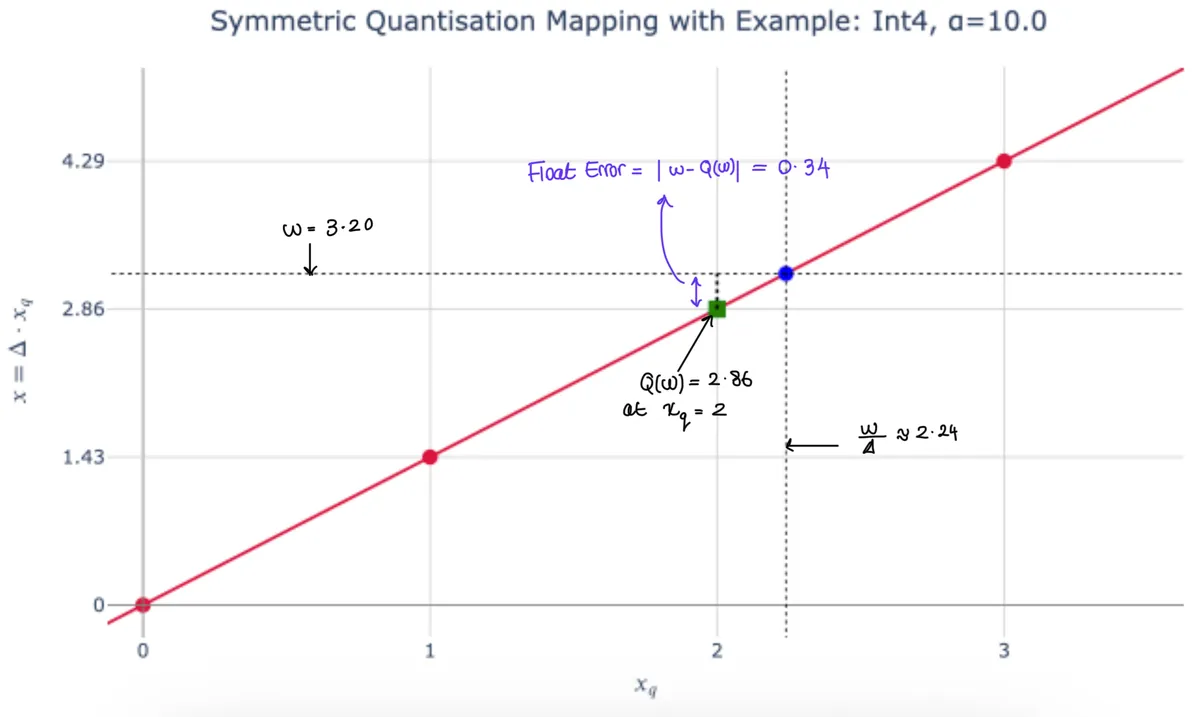
Let’s use an example for this: Suppose the quantisation step size is $Δ = 1.43$ (Same as plot above) and we have a weight with value $w = 3.2$ .

If we divide by $Δ$ to express this weight in terms of the quantisation grid, we get

\frac{w}{Δ} \approx 2.24

This tells us the weight lies a little more than two steps along the integer grid.
However, the quantiser cannot store the fractional part 0.24 as it can only keep the nearest integer code, which in this case is 2.

When we convert back to float space, the recovered (dequantised) weight is

Q (w) = 2 \times 1.43 = 2.86

The original weight was $w = 3.2$ , so the rounding mismatch in float space is

w - Q (w) = 3.2 - 2.86 = 0.34

The key insight is that the rounding happened in the scaled grid domain as we lost a fractional 0.24 step. But in the original float space, each grid step is worth $Δ$ , so that fractional 0.24 step translates into an actual error of

Δ \times 0.24 = 0.34

That’s why it's said the quantisation error is “scaled by $Δ$ ”. The size of the step determines how much any fractional misalignment in grid space costs you in real value. The larger the step size, the further apart neighbouring grid points are, so being off by a fraction of a step causes a bigger discrepancy in the recovered weight. The plot below demonstrates the example I've been going through.

📝 The plots are interactive so you can zoom into to see the float error.
I've also annotated it statically if you are interested.

Activation magnitude scaling

The formula for the output error includes a factor of $x$ which further scales the mismatch. This means the same rounding error in a weight will matter more when the corresponding activation is large, and much less when the activation is small.

Imagine for example we have two weights, $w_{1}$ and $w_{2}$ , that both suffer the same rounding error of $0.34$ after quantisation as in the previous example. The effect on the output will differ hugely based on their corresponding activations. If $x_{1} = 0.1$ and $x_{2} = 10$ :

For $w_{1}$ , the error term is $0.34 \times 0.1 = 0.034$
For $w_{2}$ , the error term is $0.34 \times 10 = 3.4$

So, in other words, the quantisation error that actually affects the network’s output isn’t just about how accurately you can store each weight; it’s about how much that weight is “used” by the input activations during inference.

Theoretical Note on Error Distribution and Activation-Awareness

The paper adds an interesting statistical observation. If you take a large collection of weights, their scaled versions $w / Δ$ tend to have fractional parts that are spread fairly evenly between 0 and 1. This means that the rounding errors, which arise when we round those fractional parts up or down to the nearest integer, are themselves uniformly distributed in the interval $[- \frac{1}{2}, + \frac{1}{2}]$ .

Since in practice we often care about the size of the error rather than its sign, it makes sense to think about the absolute value of the rounding error. Its magnitude lies in $[0, 0.5]$ , and for a uniform distribution the average absolute error works out to about 0.25 steps.

So far we have talked about the general case, that in general the quantisation error depends on both the step size $Δ$ and the input activation. That statement holds true if every weight has its own scale, because then both factors vary across weights. However, in group-wise quantisation, which is what AWQ uses, all the weights within a group share the same scale $Δ$ . This means that within a group the expected rounding error is essentially fixed, so the quantisation error in the output is proportional only to the input activation.

This is the key reason the paper refers to weight-only quantisation as activation-aware. If the activations flowing into the group are small, the quantisation error barely affects the output. If the activations are large, the same grid misalignment produces a proportionally larger discrepancy in the output. Therefore, if we could reduce the input activation magnitude in weight-only-quantisation, the quantisation error can be reduced.

Scaling Weights and Activations

Consider the same linear layer we have been using so far

y \approx Q (W) x

An intuitive idea to reduce the input activation magnitude is to scale the weights and inversely scale the activations. Let

W \in ℝ^{m \times n}, x \in ℝ^{n}, s \in ℝ^{n},

where $s$ is a vector of per-channel scaling factors. Its diagonal matrix is

d i a g (s) = [\begin{matrix} s_{1} & 0 & \dots & 0 \\ 0 & s_{2} & \dots & 0 \\ ⋮ & ⋱ & ⋮ \\ 0 & 0 & \dots & s_{n} \end{matrix}]

For a weight matrix

W = [\begin{matrix} w_{11} & w_{12} & w_{13} \\ w_{21} & w_{22} & w_{23} \\ w_{31} & w_{32} & w_{33} \end{matrix}]

multiplying by $d i a g (s)$ scales each column:

W d i a g (s) = [\begin{matrix} w_{11} s_{1} & w_{12} s_{2} & w_{13} s_{3} \\ w_{21} s_{1} & w_{22} s_{2} & w_{23} s_{3} \\ w_{31} s_{1} & w_{32} s_{2} & w_{33} s_{3} \end{matrix}]

so the $i^{th}$ column of $W$ is multiplied by $s_{i}$ . For an input activation

x = [x_{1}, x_{2}, x_{3}]

scaling by the inverse rescales the activations:

(d i a g (s))^{- 1} x = [\begin{matrix} x_{1} / s_{1} \\ x_{2} / s_{2} \\ x_{3} / s_{3} \end{matrix}]

With this re-parameterisation the layer becomes

y \approx Q (W d i a g (s)) (d i a g (s))^{- 1} x

where the scaled weights are quantised as

Q (W d i a g (s)) = Δ^{'} \cdot R o u n d (\frac{W d i a g (s)}{Δ^{'}})

and the quantisation step size is set by the maximum magnitude of the scaled weights:

Δ^{'} = \frac{max (| W d i a g (s) |)}{2^{b - 1} - 1}

In exact arithmetic this transformation does not change the computation, since

(W d i a g (s)) (d i a g (s))^{- 1} x = W x

so we are only re-parameterising the layer. However, in quantised inference the rounding now acts on the scaled weights $W d i a g (s)$ rather than on $W$ , and the quantiser’s grid is defined by the scaled magnitudes. As defined in the paper, the resulting output error is therefore

E r r (Q (W s) (\frac{x}{s})) = Δ^{'} \cdot R o u n d E r r (\frac{W s}{Δ^{'}}) \cdot \frac{x}{s}

If $s_{i} > 1$ moves $w_{i}$ closer to a quantiser grid point without increasing the group’s maximum ( $Δ^{'} \approx Δ$ ), the quantisation mismatch shrinks, and any remaining error is further reduced by the factor $1 / s_{i}$ applied to the activation. Thus, scaling allows us to reduce the effective contribution of quantisation error from the channels where it matters most.

Optimising Scaling Factors

In the paper they don’t try to optimise $s$ directly with gradients. Instead, they narrow the problem down to a simple search space, guided by the earlier point that the “importance” of a weight channel really comes from the scale of the activations flowing through it.

They write the scaling vector as

s = s_{X}^{α}

where $s_{X}$ reflects how large each input channel typically is, and $α$ is just one scalar that decides how much extra scaling we give to the big-activation channels.

The optimisation then boils down to

α^{*} = a r g {min}_{α} ℒ (s_{X}^{α})

s^{*} = s_{X}^{α^{*}}

Rather than training it, they just do a grid search over

α \in [0, 1]

When $α = 0$ there’s effectively no scaling.
When $α = 1$ you get the most aggressive scaling in this search space.

This simple setup avoids the instability of gradient-based methods and captures the key idea: channels that usually see bigger activations get scaled up more so their weights land closer to the quantiser’s grid points.

Conclusion

In summary, deploying LLMs on edge devices demands efficient compression without compromising accuracy. AWQ, a post-training group-wise weight-only quantisation technique, achieves lower quantisation error than vanilla approaches and has even outperformed more complex schemes like GPTQ, making it a practical and effective solution for running large models on memory-constrained hardware. In this blog, we explored how input activations influence quantisation errors in symmetric weight-only quantisation and demonstrated, through theoretical analysis, how making the process more activation-aware and scaling appropriately can further reduce these errors.